
Serving sub-second Ideogram v4 without quality loss




At @fal we serve Ideogram V4 at high speed. At 1K resolution, a generation that used to take 2.75 s now renders in 0.44 s, a 6x speedup with no visible quality loss. We got there by pushing the cost of a generated image down on every axis we could find, and it helps to see those axes as one equation: the cost of an image is how many forward passes the diffusion transformer runs, times how expensive each pass is.
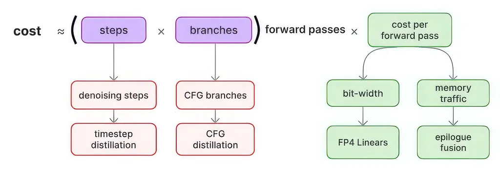
Two fronts. Make each forward pass cheap: run the transformer in FP4, and fuse the small ops around each matmul so they don't pay a memory round-trip. Make the passes fewer: distill classifier-free guidance from two branches into one, and distill the many denoising steps into a handful. Stack all of it and you land on the same image as the full bf16 model at a fraction of the compute.
This post walks the whole path, roughly in the order we built it. We start with the FP4 forward pass and the kernel fusion that makes it fast, then the quality problem 4-bit caused and the quantization-aware distillation that fixed it, and finally the timestep distillation that collapsed the step count. FP4 is fast, but naive FP4 looked visibly worse than bf16, and even then it still ran many steps times two guidance branches. Here is how we closed all of that.
Running the transformer in FP4
The fastest inference path runs the diffusion transformer in NVFP4. FP4 is a 4-bit floating point format: one sign bit, two exponent bits, one mantissa bit, so each value can only take one of a handful of levels. In exchange you get a meaningful speedup and a much smaller memory footprint, which lets us push more concurrency and lower latency per image. On Blackwell the format is supported in hardware, so the matmuls run natively in 4-bit.
But a 4-bit matmul only pays off if the matmul is where the time actually goes, and in a diffusion transformer it often isn't the whole story. Every big GEMM is chased by a small op: RMSNorm on the attention path, gated-SiLU in the FFN. Unfused, that small op forces the GEMM's entire output out to HBM and back. The matmul got cheaper, and then a memory round-trip you didn't remove eats the win. So the first thing a fast FP4 path needs is to fuse those ops into the GEMM itself.
Fusing the epilogue so FP4 pays off
Epilogue fusion, briefly
A GEMM produces A @ B in tiles. Inside each tile, Tensor Cores stream multiply-adds into an accumulator that lives in the SM's own storage: registers on Hopper, TMEM on Blackwell. While that mainloop runs, nothing has touched HBM for the output yet; the answer is being accumulated on-chip.
But A @ B is almost never the end of the layer. In a diffusion transformer the FFN is typically a GEMM followed by a gated-SiLU (SwiGLU), and the attention path by a GEMM followed by RMSNorm. The pattern repeats across LLMs and DiTs: a big GEMM, then a small post-op. The op itself is cheap; the problem is that unfused, the GEMM writes the whole tile to HBM, a second kernel loads it back, applies the op, and writes again. A few FLOPs become a full memory round-trip plus a second kernel launch.
Epilogue fusion is applying operations after the GEMM just before the result is saved to HBM. The output goes to global memory once, already transformed no second kernel, no round-trip. On Hopper and Blackwell the epilogue can overlap with the next tile's mainloop, so for small ops the extra compute is often nearly hidden.
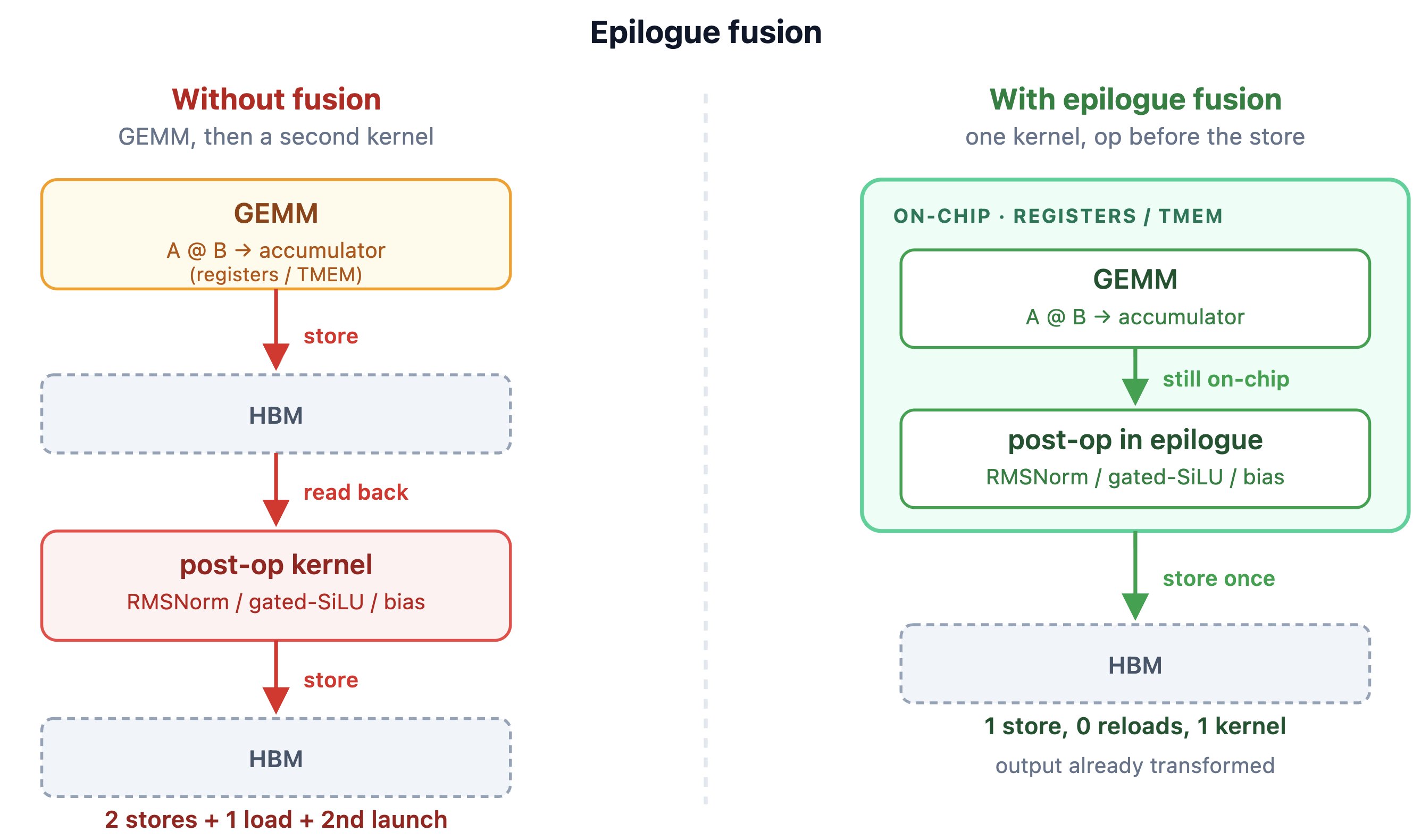
CUTLASS exposes this through Epilogue Visitor Trees (EVT). You write a visit() that runs on each accumulator fragment, and the collective epilogue handles the loads and stores. The mechanics are explained well in the Colfax EVT writeup. The short version: pointwise fusions (bias, ReLU, cast) fall out cleanly: every output element is independent, there's nothing to reduce across, and CUTLASS ships prebuilt visitors for them.
In this post we focus on fusing RMSNorm. It normalizes a vector by its own RMS: y = x · rsqrt(mean(x²) + eps) · weight. Unlike a pointwise op, it needs rstd over the whole head, a reduction. That reduction is what makes fusion hard, and to see why we need to look at how the epilogue actually sees its data.
Tiles and fragments on Blackwell
The GEMM works in CTA tiles: on Blackwell (SM100), our NVFP4 GEMM uses a 256×256 CTA tile. The epilogue doesn't process that whole tile at once; it walks it in smaller epilogue tiles of 128×128, giving 4 epilogue subtiles per CTA:
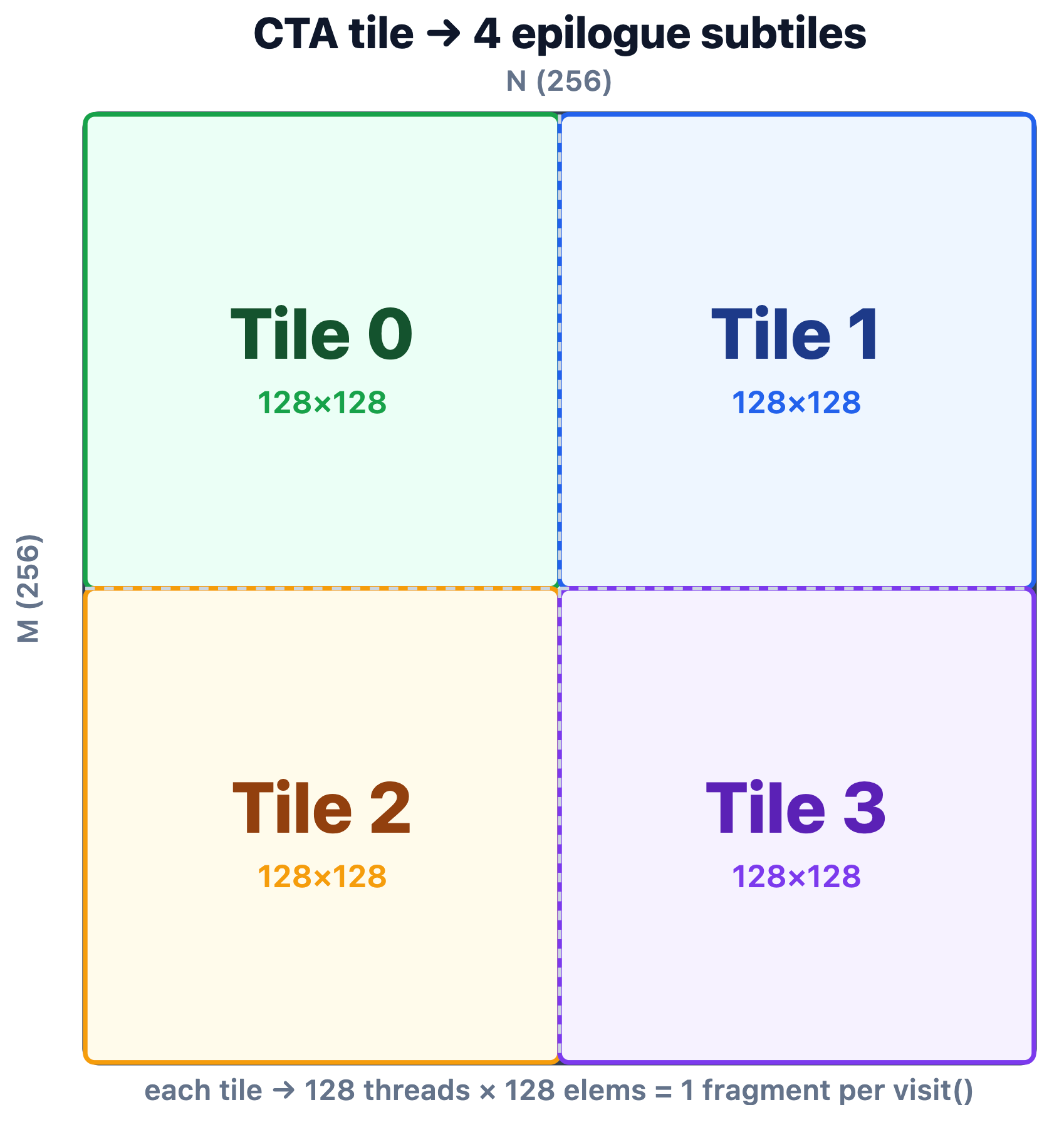
Each epilogue subtile is partitioned across 128 threads, so each thread holds a fragment of 128 elements (FragmentSize = 128). The visit() callback receives one fragment at a time, 128 values that this thread is responsible for. This is the unit of work the epilogue sees, and it matters for what you can fuse.
This makes head_dim=128 RMSNorm fusion trivial: a head of 128 elements is exactly one thread's fragment. When visit() is called, the thread is already holding all 128 values of one head in its own registers. To compute RMSNorm it sums the squares across those 128 values (no cross-thread shuffle, no second fragment, no extra pass), scales, and stores. The reduction fits in a single visit() call.
Ideogram v4 is not so convenient. Its attention uses head_dim=256, so a single head no longer fits in one fragment; it straddles two, and the clean single-visit() reduction breaks down.
Why head_dim=256 is hard
To see why that's a problem, look at how the epilogue runs. After the mainloop, CUTLASS's collective epilogue loops over the 4 subtiles of the CTA tile in a fixed order: Tile 0 → Tile 1 → Tile 2 → Tile 3, and for each subtile it calls visit() once per fragment, stores the result, and moves on. It is a single forward pass; there is no going back to an earlier subtile.
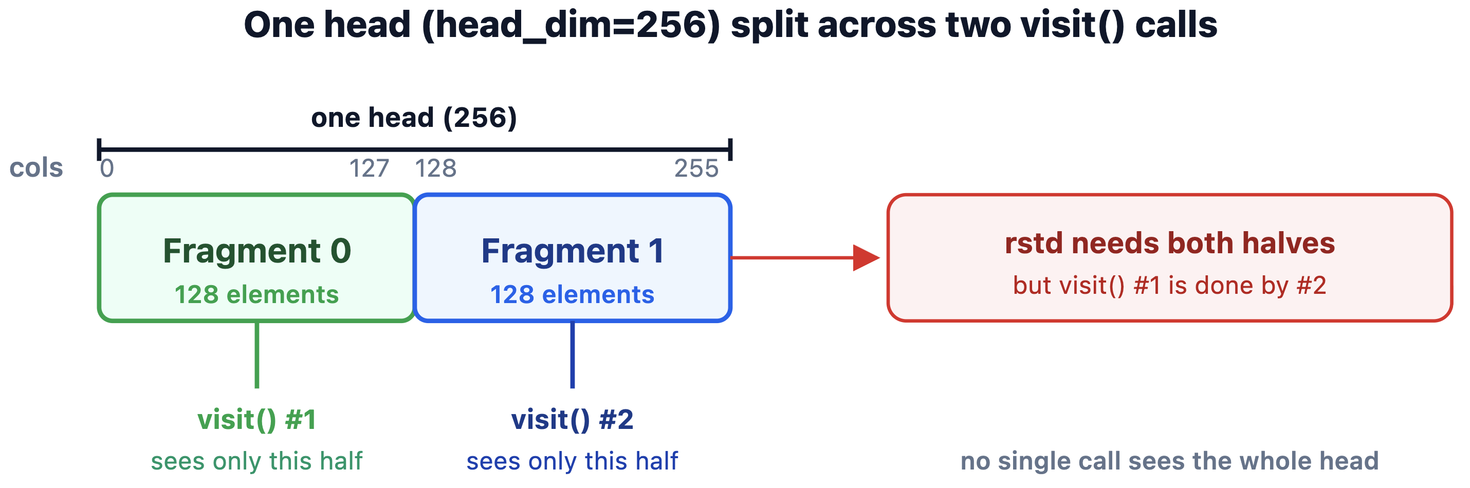
RMSNorm needs rstd over the whole head, a reduction: rstd = rsqrt(mean(x²) + eps), then y = x * rstd * weight. To compute it we need the sum of squares across both halves, but they arrive in separate visit() calls: the first half in Tile 0, the second in Tile 1. By the time we see Tile 1 and can compute rstd, Tile 0 has already been visited and stored. There's no way to go back and fix it up. The rest of this section is how we fused it anyway: a two-pass revisit schedule that keeps the first half in registers.
The revisit fusion
CUTLASS's epilogue collective works with a fixed, single-pass loop order: visit each subtile once, store, move on. That doesn't solve our problem: we need to see Tile 1 before we can normalize Tile 0, which means going back. So we wrote an epilogue that lets the visitor walk subtiles in the order the reduction needs (including coming back to a tile it already saw) instead of the stock single forward pass.
The schedule, per row-group, is three touches:
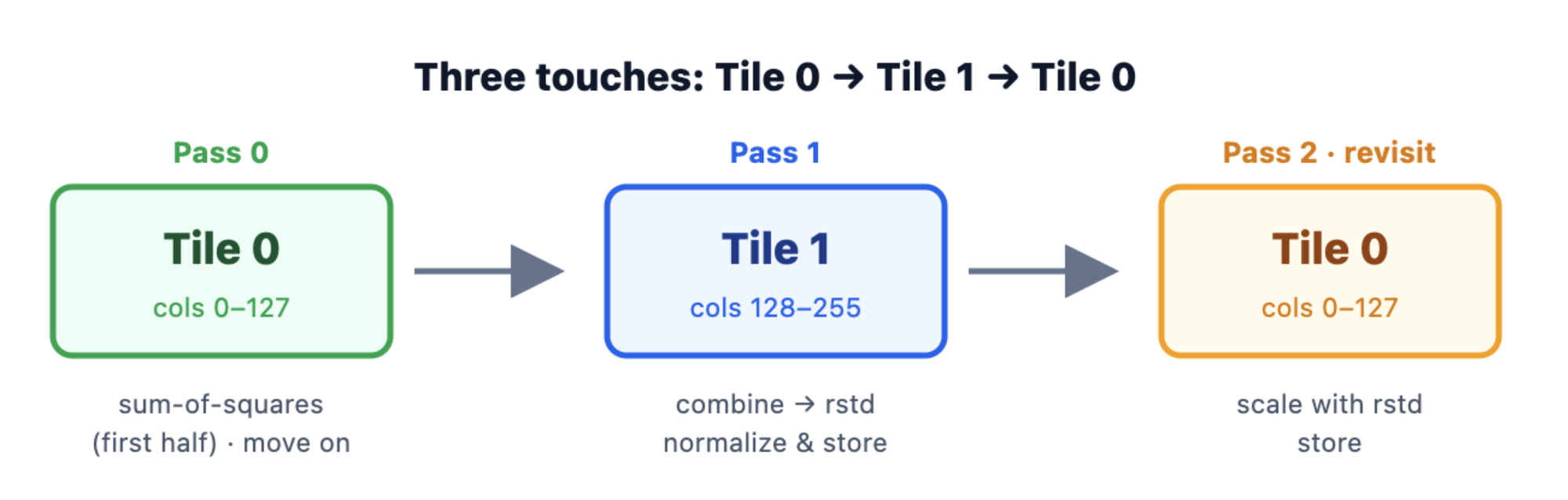
- Tile 0, pass 0: this is the first half of the head. We compute its sum-of-squares and move on; we can't normalize yet without the second half.
- Tile 1, pass 1: the second half of the head arrives. Now we have both halves: we compute this half's sum-of-squares, add it to the first half's, and finally get
rstd. We normalize and store this half. - Tile 0, pass 2 (revisit): we go back to Tile 0 and scale it with the now-known
rstd. This is the extra touch the single-pass epilogue can't do.
Everything stays on-chip: no global memory round-trip, no second kernel. A custom epilogue walks the three-touch schedule; a visitor carries the reduction state across those touches and applies the scale when rstd is ready. Together they fuse the norm before anything hits HBM.
Gated-SiLU (SwiGLU) fusion
A different common pattern in diffusion transformers (and LLMs like LLaMA) is gated-SiLU. One GEMM produces an output C, then the layer finishes by splitting it in half and multiplying:
C = A @ B
output = SiLU(C[:, :N//2]) * C[:, N//2:]
That cuts the output width in half; two halves become one. Same story as RMSNorm: the math is cheap, but an unfused second kernel pays a full HBM round-trip. CUTLASS has no built-in epilogue for this "pair + reduce N/2" pattern, so fusing it means a custom visitor.
The catch is layout. For output column n, the pair is gate = C[:, n] and up = C[:, n + N/2], separated by half of N. Those two values can easily land in different fragments, different subtiles, or even different CTAs. Synchronizing across tiles would kill the epilogue's parallel model.
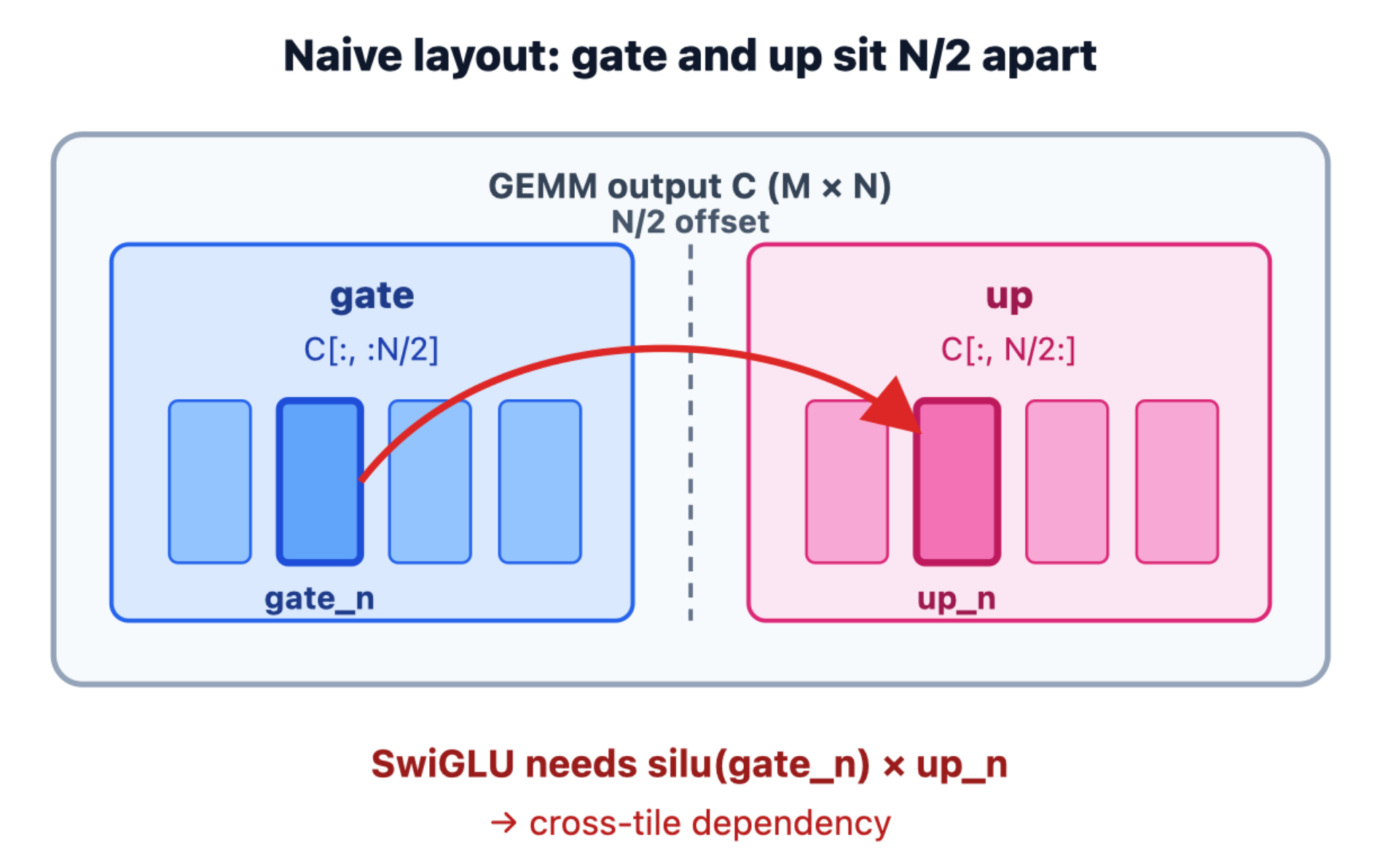
Instead we permute the columns of B once during weight packing. The GEMM then produces interleaved pairs [gate0, up0, gate1, up1, ...] instead of two separated halves. With adjacency guaranteed, a custom EVT visitor applies SiLU and the multiply on adjacent elements in the same fragment, and stores the reduced result: one kernel, no cross-tile communication.
The full walkthrough (weight packing, the visitor hooks, and the EVT wiring) is in Crafting Efficient Kernels with Epilogue Fusion.
The catch: FP4 costs image quality
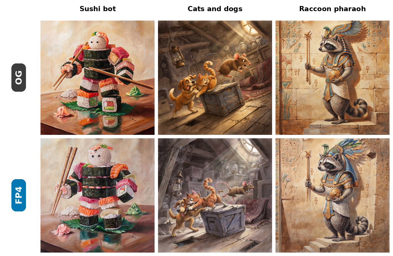
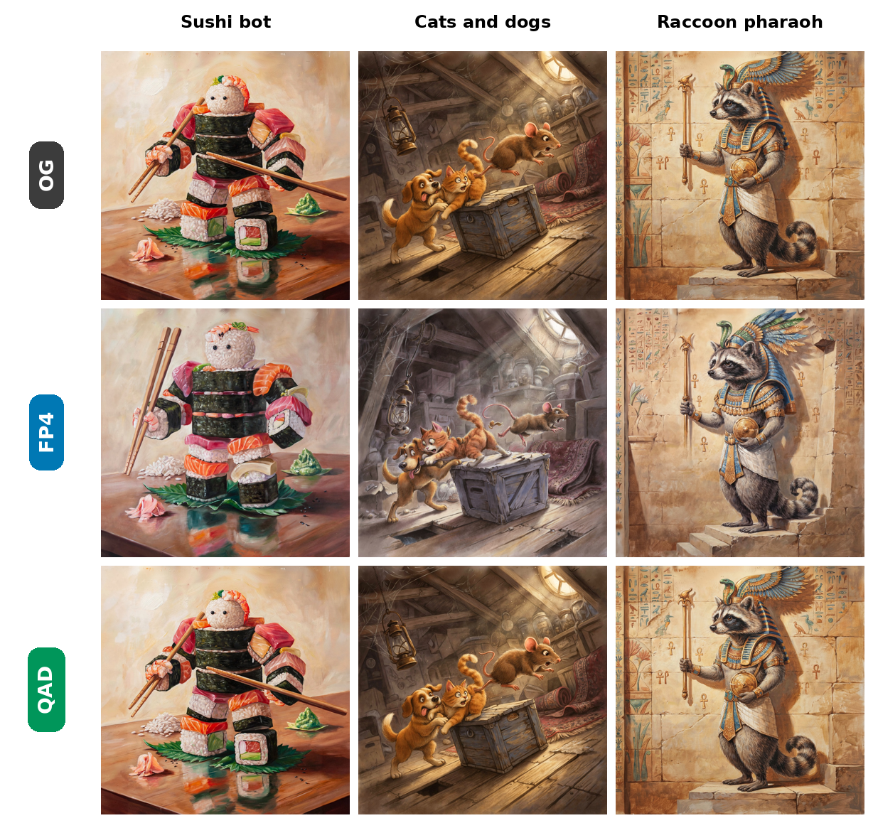
Fusing the epilogue gets us a fast FP4 forward pass. On its own, it also gets us a worse-looking one. Stock FP4 inference looked visibly worse than bf16, specifically on color. Reds washed out, chroma dropped, and color-heavy prompts (logos, products, plants) looked desaturated next to the bf16 reference.
Those handful of levels per value are fine for a large language model, where every token is a small contribution to a big average. A diffusion transformer is less forgiving, because it iteratively denoises a latent over many steps and each step feeds its output into the next. A slightly wrong velocity at one step becomes a wrong latent at the next, which feeds a wrong input at the step after that. The error snowballs. With FP4, this compounding showed up as desaturation: the model still produced the right composition, but colors came out flatter and less vivid than the bf16 model.
Post-processing tricks (luma correction, color rebalancing) did not materially help, because the error was baked into the latents before decoding, not just a display-space issue. We needed to fix this inside the model, not after it.
What did not work
Before landing on the final recipe, we tried a few things that taught us what matters and what does not:
- Post-processing on the output. Our first instinct was to just fix the colors after generation. Saturation correction, luma adjustment, color rebalancing on the decoded image. None of it worked. The desaturation is not a display problem; it is a latent trajectory problem. By the time you have pixels to correct, the denoiser has already taken slightly wrong steps for many iterations, and the color information is just gone. You cannot un-bake it from the final image.
- Naive distillation. We tried the simplest thing: quantize the student to FP4, run a bf16 teacher on the same input, and minimize MSE between their predictions. No gradient flowed through the quantization - the student was frozen in its quantized state and just compared to the teacher. Loss went down, images did not get better. That is when we learned the hard way that diffusion training loss does not predict image quality. You can watch it drop for thousands of steps and the output barely changes.
These told us two things: the quantization error had to be addressed during training (not after), and the final judgment had to be visual (not numeric).
Quantization-aware distillation
Around the time we were wrestling with this, a technique called quantization-aware distillation (QAD) was published for LLMs and VLMs(paper). The idea is simple in hindsight: instead of just quantizing a model and hoping for the best, you distill a full-precision teacher into a quantized student. The student learns to predict what the teacher would have predicted, but under the constraint of its own quantization noise. The teacher is frozen bf16, the student is quantized, and you train the student to match the teacher's output.
That paper used KL divergence on logits, because it was about LLMs. We are not predicting tokens; we are predicting a velocity field over a latent. So we swapped the loss: MSE between the student's velocity prediction and the teacher's velocity prediction. Same spirit, different objective.
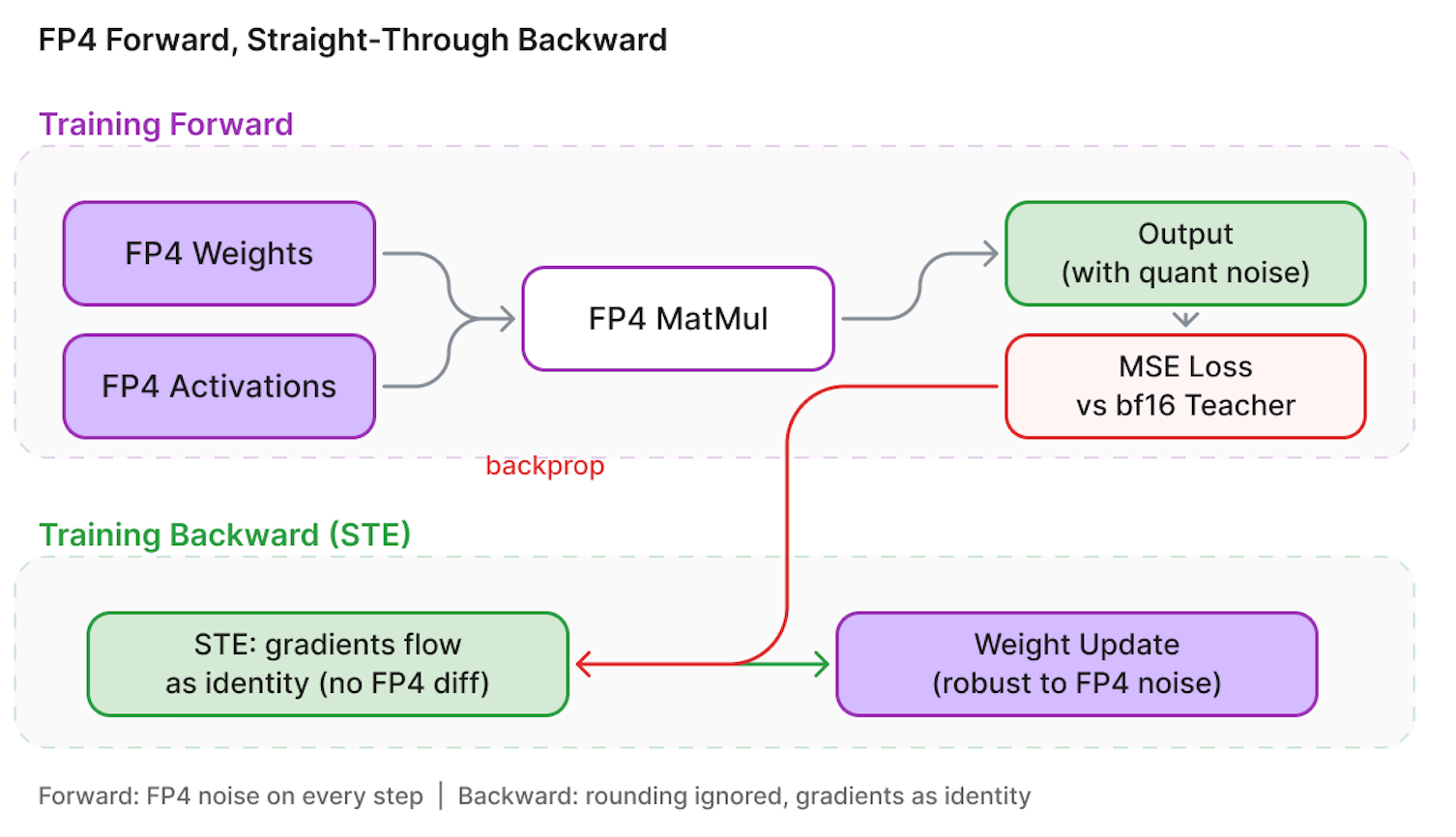
The critical difference from the naive distillation we tried earlier: in QAD, the student does not just run in FP4 and get compared to a teacher. The student trains through its own quantization. Gradients flow back through the FP4 rounding via a straight-through estimator, so the weights actively adapt to the quantization noise they produce. That is the whole point - the weights move to a part of parameter space where being rounded to 4 bits does not hurt the output. Naive distillation just compares a frozen-quantization student to a teacher and hopes; QAD lets the quantization be part of the optimization.
In the forward pass, the student's bf16 weights and activations are quantized to FP4 for the matmul, then dequantized back. The output carries real quantization noise from that round-trip. The frozen bf16 teacher produces the target velocity. The loss is MSE between the student's noisy prediction and the teacher's clean target. In the backward pass, the FP4 rounding is detached from the autograd graph: a rounding function has zero gradient almost everywhere, so it cannot be differentiated directly, and the straight-through estimator simply bypasses it, letting gradients flow in full precision. The forward pass carries the quantization noise; the backward pass ignores it. Over training, the weights converge to a region of parameter space where rounding to 4 bits does not degrade the output.
At inference, none of this is needed. We export the trained weights, load them into the production pipeline, apply real static FP4 quantization with the real kernels, and generate images. The student runs as just the conditional branch with guidance = 1 - no teacher, no CFG, no STE.
Collapsing CFG into one forward
Classifier-free guidance (CFG) is how diffusion models steer toward the prompt. At inference, you run the transformer twice per step: once conditioned on the prompt (conditional), and once with no text (unconditional), That is a 2x cost on every denoising step. We realized we could fold this into the distillation and get it for free.
During training, the frozen bf16 teacher runs both branches and produces the guided CFG velocity. The student is only the conditional branch, and it is trained to directly predict that guided velocity. At inference, we run the trained conditional branch alone with guidance = 1 - one forward pass instead of two. So on top of the FP4 speedup, we halve the transformer cost by removing CFG entirely from the serving path.
This is the part that goes beyond the QAD paper. That paper recovers quantization accuracy and stops. We recover quantization accuracy and distill away the CFG branch, so the final inference graph is both smaller (fp4) and shorter (one branch).
What made QAD work
Getting QAD to actually recover visual quality required a few decisions beyond the core recipe. These are the ones that mattered most:
- Loss combination. We use flow-matching loss in combination with distillation loss to utilize real data quality. Pure distillation alone was not enough to recover the full visual quality we wanted.
- Guidance schedule. We did not use one fixed guidance for the teacher target. We used higher guidance over the noisy and mid timesteps and lower guidance near the clean end, because the model benefits from stronger steering early and gentler steering as it converges.
With QAD recovering the quality and CFG folded into a single branch, two of the three cost multipliers are handled. The last one is the biggest.
Timestep distillation
We have now made each forward pass about as cheap as it gets: 4-bit matmuls in FP4, fused epilogues so the norms and activations don't pay a round-trip, and a single guidance branch instead of two. The one thing we haven't touched is how many forward passes there are, the number of denoising steps, and it is the biggest lever of all.
A diffusion transformer earns its quality by denoising a latent over many iterations, and every iteration is a full forward pass. If you can teach the model to do the same job in a handful of steps, you collapse the single largest factor in latency and throughput. That is timestep distillation. It is also the part of the pipeline with the most moving parts, the most literature, and the most ways to quietly ruin image quality.
The foundation: Distribution Matching Distillation
The natural first idea is regression: run the teacher, run the student, minimize the MSE between them. That is what the QAD work above does, and it works when the student and teacher take the same path. But a few-step student does not take the same path as a many-step teacher. You cannot ask it to hit the same intermediate latents, because it is skipping most of them. Regression pins the student to a trajectory it should be free to leave.
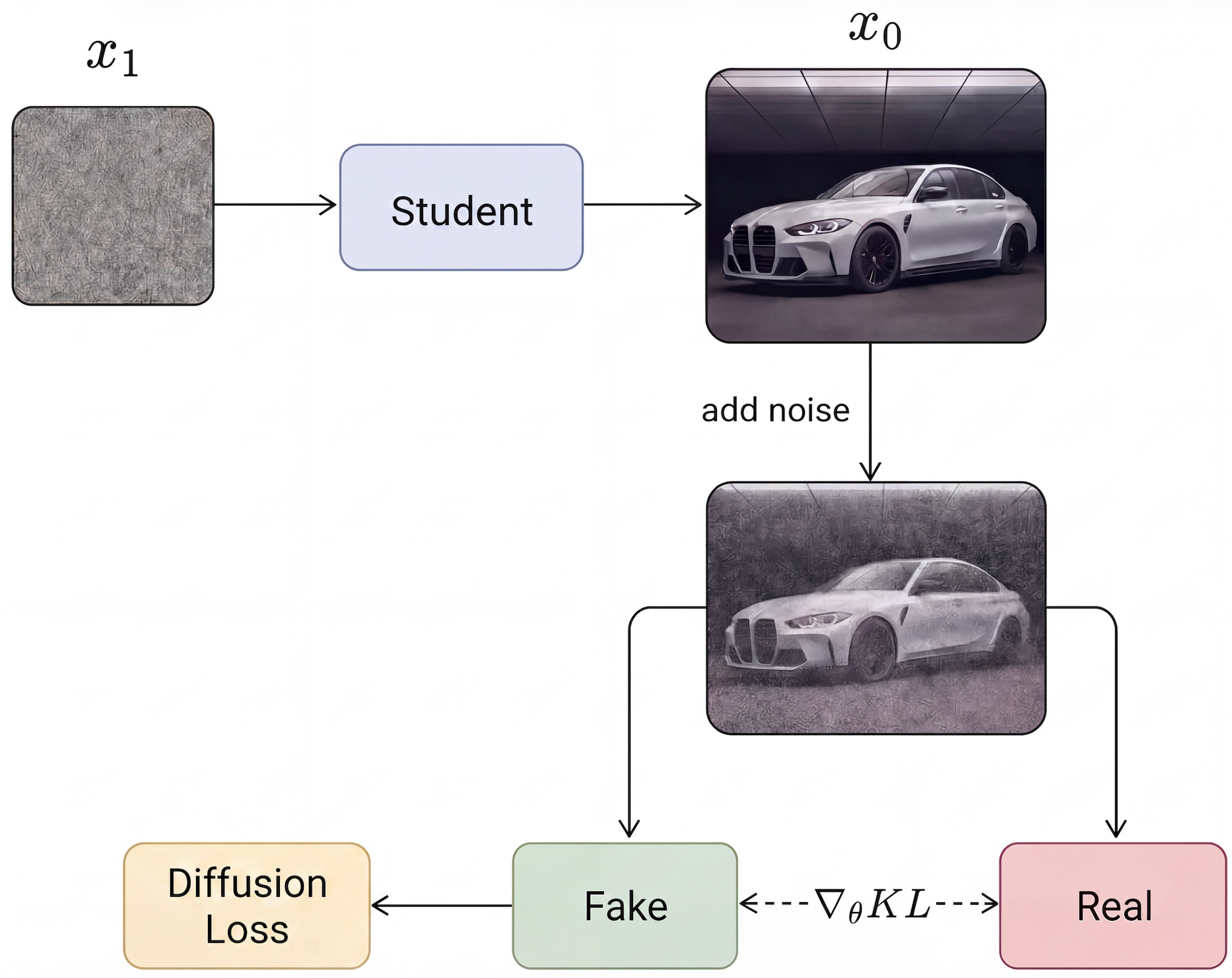
Distribution Matching Distillation (DMD) reframes the goal: instead of matching the teacher sample by sample, match distribution to distribution. We don't care what the student does on any single trajectory; we care that the cloud of images it produces looks like the cloud the teacher produces.
The mechanism keeps two score networks: a real score (the frozen teacher) and a fake score (a second network tracking the student's current distribution). To update the student, DMD takes a student sample, renoises it, and asks both score networks where to go. The difference between the two scores is a gradient direction that moves the student's distribution toward the teacher's. That difference-of-scores is, up to a constant, the gradient of the KL divergence between the two distributions at that noise level. No paired targets, no MSE to a specific latent, just "make these two distributions agree."
DMD2: the version people actually ship
DMD2 cleans up vanilla DMD into the recipe most modern few-step image models descend from: it drops the regression term (making the method data-free), uses two-timescale updates so the fake score stays accurate as the student changes, adds a GAN loss as a secondary sharpening term, and supports multi-step sampling so the student isn't locked to a single step count.
A whole family, each chasing a different lever
DMD2 kicked off a family of follow-ups. The right choice depends on what you're optimizing for: DMDR, Flash-DMD, AdvDMD, and GNDM fold RL and reward signals into distillation. DP-DMD preserves diversity. AMD improves stability. Decoupled DMD shows the guidance term is the real engine while distribution matching acts as a regularizer.
The branch closest to our work is trajectory and off-trajectory matching. Training stability was a real concern: the GAN loss is the fragile part of DMD2, so we wanted to get as far as possible without a discriminator. That pushed us toward GAN-free, data-free distribution matching. The two closest public methods:
- TDM matches distributions at points along the teacher's trajectory, with a sampling-steps-aware objective so one model works across several step counts. It stays on the trajectory; its flexibility comes from being steps-aware.
- CDM goes off-trajectory, enforcing distribution matching on extrapolated latents from the student's own velocity field, keeping it robust when the schedule changes.
Our own objective is a custom, GAN-free, data-free, distribution-matching design in the same spirit. The goal was a stable distillation that reaches high quality and stays flexible across step counts, not any single published recipe.
First, distill without a GAN
We did the first pass GAN-free: just our custom distribution-matching objective, no discriminator. This gave us a few-step student that was genuinely good, with the right composition, faithful prompt following, and stable behavior across a flexible step schedule. On most prompts you would be hard pressed to tell it from the teacher. It just wasn't quite production-grade. The last increment of sharpness and fine-texture fidelity wasn't there yet. Distribution matching gets the distribution right; squeezing out the final per-sample crispness is a different job.
Then add the GAN
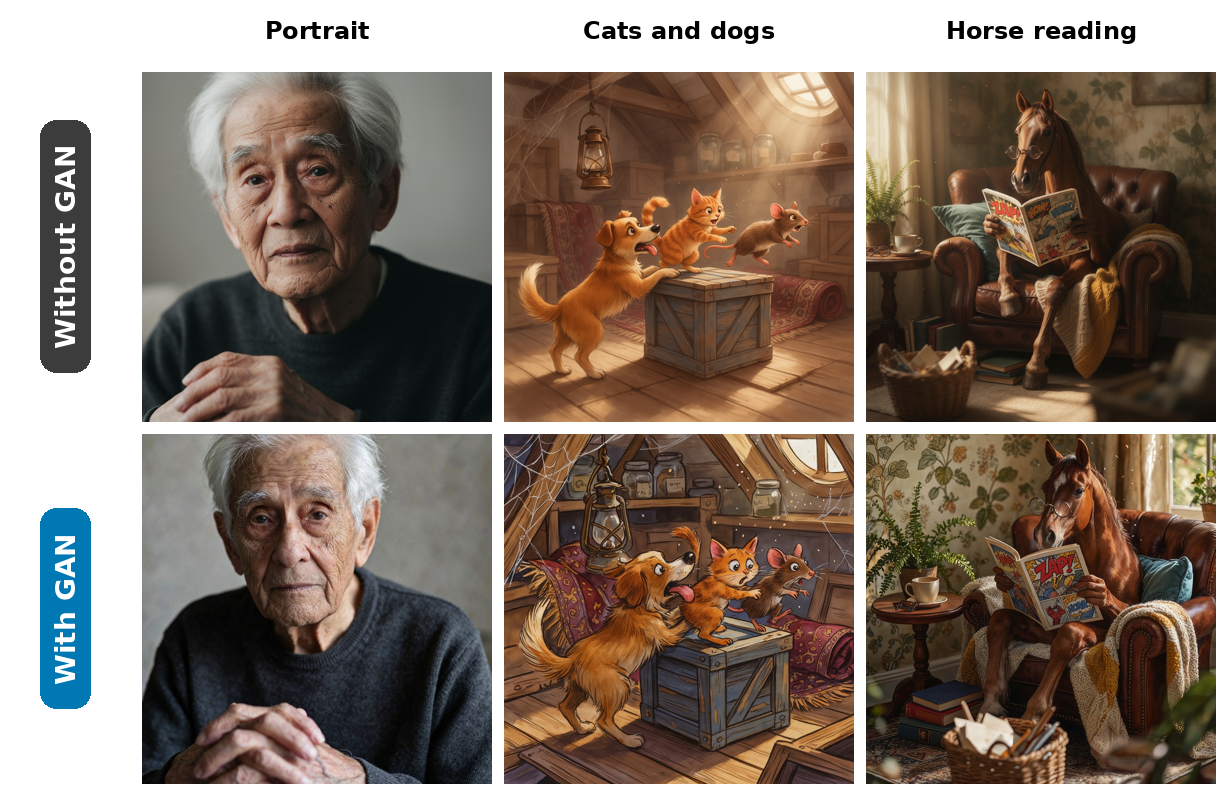
A discriminator fed real data knows what "crisp and real" looks like better than any score approximation. The problem with adversarial training is that it usually collapses when the student starts weak: the discriminator wins instantly, gradients saturate, and the generator never learns. Most of the literature spends effort handicapping the discriminator with approximate R1 regularization (as in APT) or random projections, which is what we used in our earlier FLUX.2 dev Turbo distillation.
For this model we used no stabilizer at all, and didn't need one. Because we start from the already-strong distilled student, its samples are close to real from step one, so the discriminator never gets the free win that causes collapse. Training stays stable on its own, and the GAN recovers the last of the sharpness and detail.
This is the opposite of how DMD2 uses adversarial loss, where DMD2 layers the GAN as a secondary term. For us it is the primary post-training objective, and it works because the student it starts from is already strong. A recent two-step method explore similar idea of using GAN as a post-training loss.
Back to FP4
The few-step student is bf16. To serve it, we run it through the same QAD path: quantization-aware distillation against the now-few-step teacher, STE, export, real FP4 static quantization. The final model is few-step, 4-bit, and single-branch - no CFG to fold this time, since the few-step student is single-branch by construction.
Where this leaves us
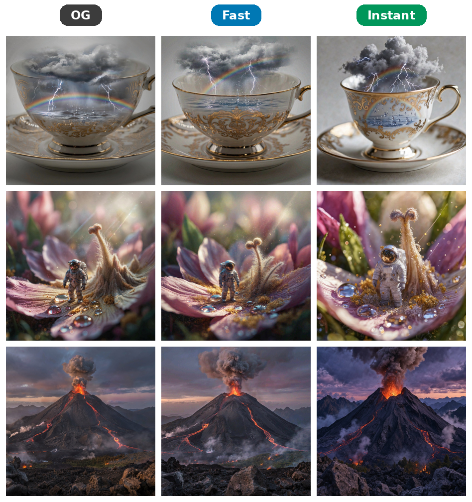
The final serving path is a few-step, single-branch, FP4 model with fused kernels. Each technique tackles a different part of the cost equation, and they stack: FP4 and epilogue fusion make each forward pass cheap, CFG distillation halves the branches, timestep distillation cuts the steps, and QAD recovers the quality lost to 4-bit quantization. The result is an image model that lands on the same output as the many-step bf16-with-CFG sampler at a fraction of the compute, with no visible quality loss on the prompts that used to break stock FP4.
Both production tiers run this FP4 path, which is a big part of why they beat the bf16 baseline. At 1K resolution:
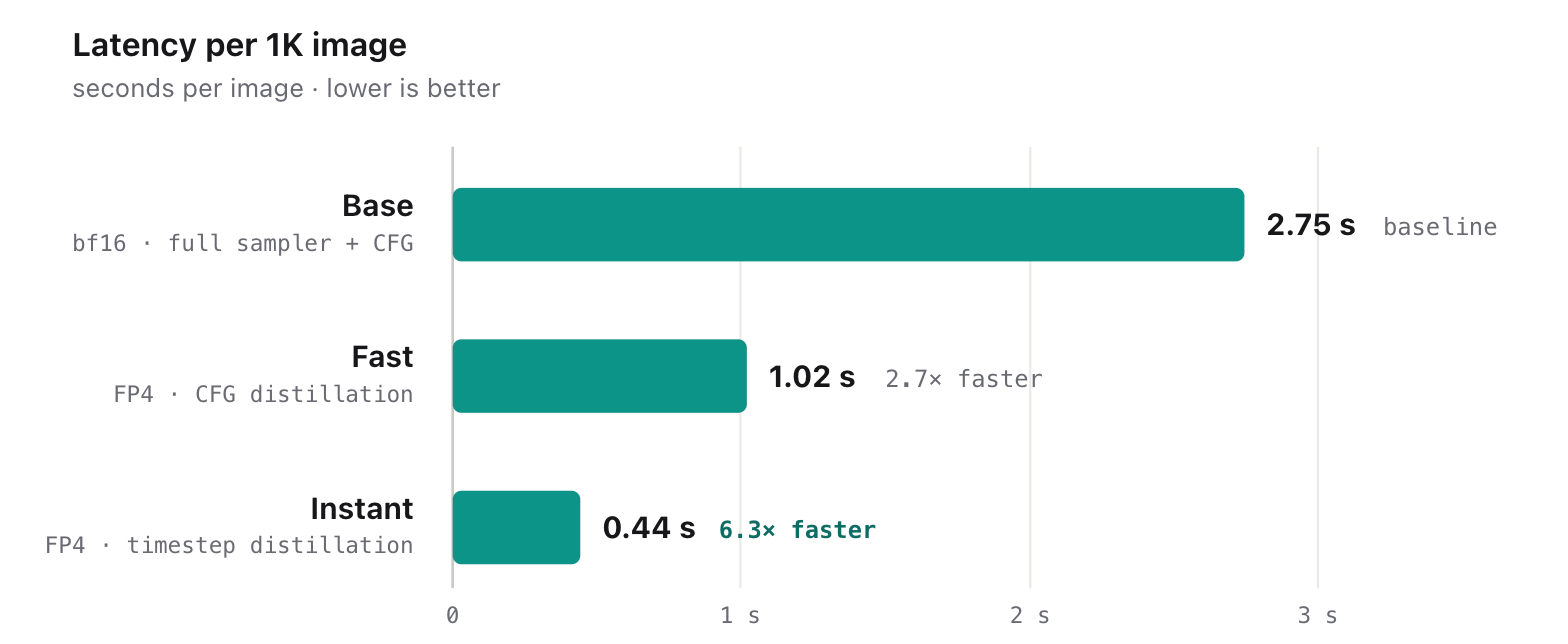
Fast collapses the two guidance branches into one; Instant collapses the step count on top, landing 6.3× faster than Base.