Instruction-level control with Inline Elementwise ASM in Triton


Triton is a DSL (Domain-Specific Language) which makes it deceptively easy to write fast GPU kernels in Python since it abstracts all the nuances of writing a pure GPU kernel from scratch, such as manual memory hierarchy handling, synchronization, and low-level launch configuration while still producing highly optimized GPU code.
However, the moment you want exact control over the device specific assembly instructions that a Triton kernel might not generate like packing bits, using special/faster instructions, and so on, you hit a wall. This wall is usually where people drop down to a lower level where one can write any kind of assembly instruction they want.
To overcome this wall, Triton provides a middle ground API: inline elementwise assembly
In this blog post, I'll show how Triton lets you inject elementwise GPU assembly instructions without ever leaving the comfort of Python and when this approach is actually worth it. Let's first understand, in short, what a Triton kernel actually compiles to. Note, this post will focus purely on NVIDIA GPUs where the device specific assembly is also called PTX.
From Python to PTX
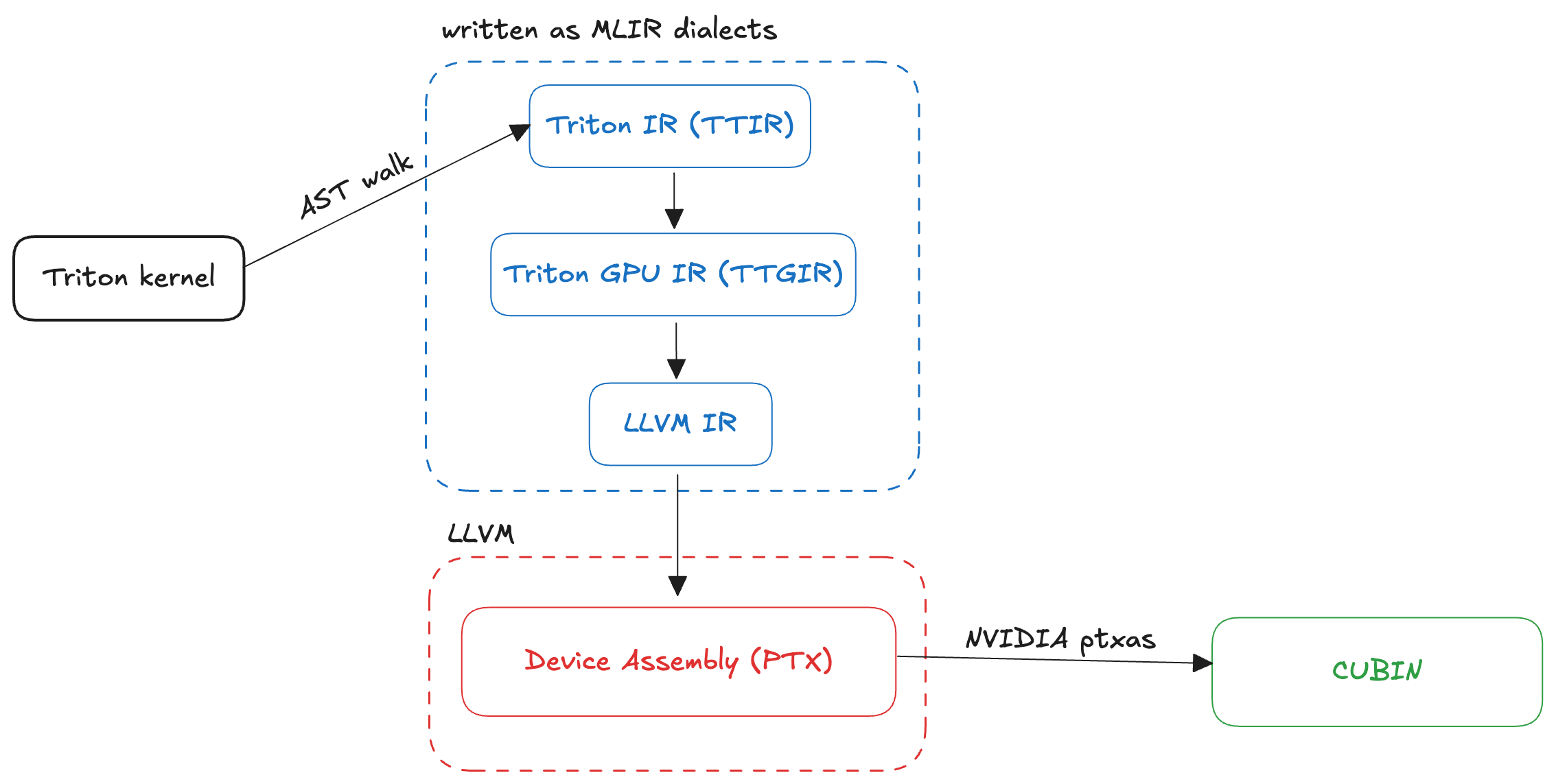
Triton lowers from Python to device specific assembly through many lowering stages. A brilliant article by Kapil Sharma summarizes what exactly happens during a Triton kernel compilation:
- Python kernels are parsed into a high-level Triton IR representing tensor and kernel semantics.
- The IR is progressively lowered through MLIR dialects (Triton -> TritonGPU -> TritonNVIDIAGPU), where domain-specific optimizations such as tiling, vectorization, CSE, and constant folding are applied.
- The optimized Triton IR is lowered to LLVM IR, enabling further compiler optimizations.
- LLVM IR is translated to PTX, NVIDIA’s GPU intermediate representation.
- PTX is JIT-compiled by NVIDIA’s toolchain into a CUBIN, which is executed on the GPU.
The image below gives a visual representation of what happens during Triton kernel compilation:
Next, let's see an example of injecting a single elementwise PTX instruction within a Triton kernel.
Example 1: single instruction (rcp)
Triton provides us with the inline_elementwise_asm function through which we can inject a PTX instruction that works in an elementwise manner on some given arguments. The signature of the function is as follows:
triton.language.inline_asm_elementwise(asm: str, constraints: str, args: Sequence, dtype: dtype | Sequence[dtype], is_pure: bool, pack: int, _semantic=None)
I'll explain the arguments this function takes throughout this blog post but let's focus on the following example.
Suppose, we are given two float32 matrices A and B of shape (M, N) and we want to compute another matrix C of the same shape where:
ci = ai / bi
This operation is readily available in Triton for the float32 data type. However, we can compute the result in another way too:
ci = ai * (1 / bi)
Here (1 / bi) is just the reciprocal of the bi value. Keep this in mind.
A normal Triton kernel, without any inline PTX, for this operation will look something like:
@triton.jit
def _kernel(
    a_ptr, b_ptr, c_ptr, N,
    BLOCK_SIZE: tl.constexpr = 1024
):
    pid = tl.program_id(0)
    offs = pid * BLOCK_SIZE + tl.arange(0, BLOCK_SIZE)
    mask = offs < N

    a = tl.load(a_ptr + offs, mask=mask, other=0.0)
    b = tl.load(b_ptr + offs, mask=mask, other=1.0)

    c = a / b
    tl.store(c_ptr + offs, c, mask=mask)
The host function for this kernel will be:
def div(a: torch.Tensor, b: torch.Tensor, version=1):
    numel = a.numel()
    out = torch.empty_like(a)

    grid = lambda meta: (triton.cdiv(numel, meta['BLOCK_SIZE']), )
    K = _kernel[grid](a, b, out, numel, BLOCK_SIZE=1024)
    return out, K
We can inspect the Triton compiled PTX of this kernel by dumping K.asm['ptx'] in a file. When we do that, we see Triton uses the following instruction to compute ai / bi in the PTX:
div.full.f32 d, a, b;
Here, the value ai is stored in the 32-bit register a, value bi is stored in the 32-bit register b, and the result in d.
When we look at the PTX docs we find an instruction that computes a fast approximate reciprocal of a given float32 value:
rcp.approx{.ftz}.f32 d, a;
So, if we want, we can compute a fast approximate reciprocal of the bi value and then multiply the result with the ai value. To do this, we need to update the kernel as follows:
@triton.jit
def _kernel(
    a_ptr, b_ptr, c_ptr, N,
    BLOCK_SIZE: tl.constexpr = 1024
):
    pid = tl.program_id(0)
    offs = pid * BLOCK_SIZE + tl.arange(0, BLOCK_SIZE)
    mask = offs < N

    a = tl.load(a_ptr + offs, mask=mask, other=0.0)
    b = tl.load(b_ptr + offs, mask=mask, other=1.0)

    (multiplier,) = tl.inline_asm_elementwise(
        asm="rcp.approx.ftz.f32 $0, $1;",
        constraints="=r,r",
        args=[b],
        dtype=[tl.float32],
        is_pure=True,
        pack=1
    )
    c = a * multiplier
    tl.store(c_ptr + offs, c, mask=mask)
In essence, this is a map over the elements of a Triton tensor where the function is inline PTX.
asm: This is the string instruction which will be used over the elements of a tensor. To access the elements as 32-bit registers, we can use the placeholders$0,$1,$2and so on.constraints: This is a string which tells Triton the number of output and input registers based on the number of input and output tensors and dtypes respectively. To get more idea, take a look at ASM LLVM format documentation. Output registers are identified with=rand input registers arer.args: The input Triton tensors, whose values are passed to the inline assembly block as 32-bit registers.dtype: The element type(s) of the returned tensors. It is on the programmer to correctly configure the output registers and their dtypes to avoid incorrect results.is_pure: If true, the Triton compiler assumes the ASM block has no side-effects and the inline ASM works as it is.pack: Each invocation of the inline asm processes pack elements at a time. Exactly which set of inputs a block receives is unspecified. Input elements of size less than 4 bytes (32-bits) are packed into 4-byte (32-bit) registers.
In this example, since we are only dealing with float32 dtype, we don't need any packing and we only handle one element at a time.
When we run both the versions, we see no difference in the outputs but when we inspect the PTX generated by Triton here's what we see:
PTX generated by version 1
div.full.f32 	%r33, %r1, %r17;
div.full.f32 	%r34, %r2, %r18;
div.full.f32 	%r35, %r3, %r19;
div.full.f32 	%r36, %r4, %r20;
div.full.f32 	%r37, %r9, %r25;
div.full.f32 	%r38, %r10, %r26;
div.full.f32 	%r39, %r11, %r27;
div.full.f32 	%r40, %r12, %r28;

Execution time: 0.12382 ms
PTX generated by version 2
rcp.approx.ftz.f32 %r33, %r34;
rcp.approx.ftz.f32 %r35, %r36;
rcp.approx.ftz.f32 %r37, %r38;
rcp.approx.ftz.f32 %r39, %r40;
rcp.approx.ftz.f32 %r41, %r42;
rcp.approx.ftz.f32 %r43, %r44;
rcp.approx.ftz.f32 %r45, %r46;
rcp.approx.ftz.f32 %r47, %r48;
mul.f32 	%r49, %r33, %r1;
mul.f32 	%r50, %r35, %r2;
mul.f32 	%r51, %r37, %r3;
mul.f32 	%r52, %r39, %r4;
mul.f32 	%r53, %r41, %r9;
mul.f32 	%r54, %r43, %r10;
mul.f32 	%r55, %r45, %r11;
mul.f32 	%r56, %r47, %r12;

Execution time: 0.12375 ms
Infact, the second version is a bit faster than the first one! Apart from that, injecting elementwise PTX gives us a lot more flexibility when we need to play with bit packing, special instructions, and so on than regular Triton.
Example 2: packing and multiple instructions
Suppose we have two float16 arrays A and B of shape (N,) and we want to compute C and D as follows:
ci = ai * bi + 1.0
ci = clamp(ci, 0.0, 6.0)
di = ci * ci
Since the dtype here is float16 we can use the elementwise assembly function to handle 2 elements at once. Triton will implicitly pack two float16 values in one 32-bit register. Along with this, we can use the following f16x2 PTX instructions to compute C and D:
fma.rnd{.ftz}{.sat}.f16x2   d, a, b, c;
max{.ftz}{.NaN}{.xorsign.abs}.f16x2    d, a, b;
mul{.rnd}{.ftz}{.sat}.f16x2 d, a, b;
The normal and PTX injected kernels look like:
@triton.jit
def kernel_fp16_normal(A, B, C, D, BLOCK: tl.constexpr):
    offs = tl.program_id(0) * BLOCK + tl.arange(0, BLOCK)
    a = tl.load(A + offs)
    b = tl.load(B + offs)

    y = a * b + 1.0
    y = tl.clamp(y, 0.0, 6.0)

    tl.store(C + offs, y)
    tl.store(D + offs, y * y)
and,
@triton.jit
def kernel_fp16_pack2(A, B, C, D, BLOCK: tl.constexpr):
    offs = tl.program_id(0) * BLOCK + tl.arange(0, BLOCK)
    a = tl.load(A + offs)
    b = tl.load(B + offs)

    (c, d) = tl.inline_asm_elementwise(
        asm="""
        {
            .reg .b32 tmp<3>;
            mov.b32 tmp0, 0x3C003C00;  // 1.0
            mov.b32 tmp1,  0x00000000;  // 0.0
            mov.b32 tmp2,   0x46004600;  // 6.0

            // y = a * b + 1
            fma.rn.f16x2 $0, $2, $3, tmp0;

            // clamp
            max.f16x2 $0, $0, tmp1;
            min.f16x2 $0, $0, tmp2;

            // d = y * y
            mul.rn.f16x2 $1, $0, $0;
        }
        """,
        constraints="=r,=r,r,r",
        args=[a, b],
        dtype=(tl.float16, tl.float16),
        is_pure=True,
        pack=2,
    )

    tl.store(C + offs, c)
    tl.store(D + offs, d)
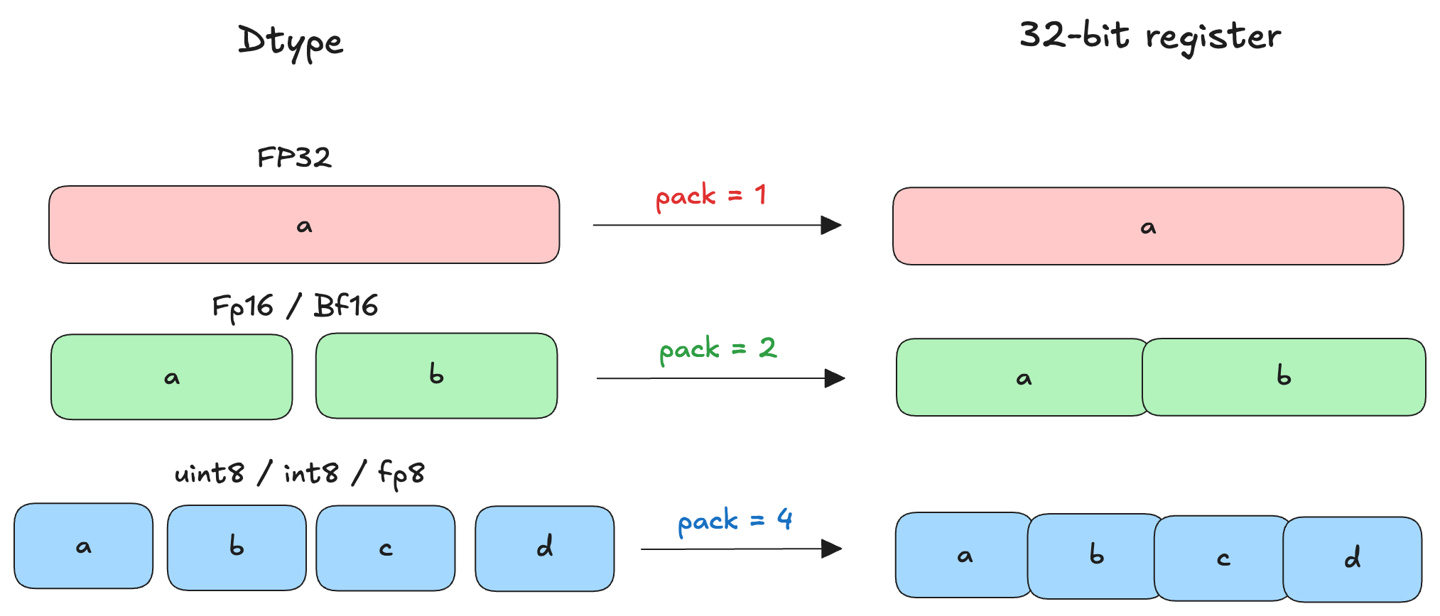
Here, we pass the two Triton tensors as arguments. We use the value of pack as 2 so that Triton can pack two float16 elements in one 32-bit register which we can use with the f16x2 instruction. For the outputs, Triton also unpacks the 32-bit register containing the f16x2 value (32-bit register) to the given output dtype.
The below image shows how packing elements will work with different dtypes:
When we compare the outputs, we see no difference but when we look at the effective memory bandwidth (in GB/s) achieved by both the kernels, we get:
Normal Triton   : 6502.08 GB/s
Inline PTX f16x2: 6514.12 GB/s
The second kernel that uses inline PTX seems to be 12 GB/s faster than the first kernel in this example!
In the above toy examples, Triton already provides support for the operations we want. However, let's look at a real-world example now to understand that we can use PTX instructions even when Triton does not provide an explicit support for them out of the box.
Example 3: NVFP4 quantization on Blackwell GPUs
NVFP4 is a block-scaled quantization recipe that quantizes a given matrix X of shape (M, N) to FP4 e2m1 dtype. Given the narrow precision of FP4, to mitigate the quantization error we use two scale factors here: Global tensorwise scale (with dtype fp32) and Local block scale (with dtype FP8 e4m3). The block scale size here is 16 i.e. every consecutive 16 elements share a local scaling factor.
I won't be going into the details of how exactly to quantize a matrix X of shape (M, N) to NVFP4 i.e. fp4 e2m1 dtype but the gist is:
- Compute the global absolute maximum value across the tensor (amax_x).
- Compute the global encode scale as (6 × 448) / amax_x, and store its inverse as the global decode scale in FP32.
- Split the tensor into contiguous blocks matching Tensor Core granularity.
- For each block, compute the block absolute maximum (amax_b) and the local decode scale as amax_b / 6.
- Multiply the local decode scale by the global encode scale and quantize it to FP8 (E4M3) using round-to-nearest-even.
- Recover the effective local encode scale by inverting the quantized FP8 decode scale and applying the global decode scale.
- Scale each value in the block using the local encode scale and quantize it to FP4; store FP4 values along with FP8 local decode scales and FP32 global decode scale for GEMM.
The thing is: if we were to write this quantization recipe in terms of PyTorch we would have to play around with bit manipulation and bit packing operations. The below pseudocode shows how the function would look like:
function QUANT_NVFP4(x):
    assert last_dim(x) % 16 == 0

    x_blocks <- reshape x into (..., N/16, 16) as FP32

    if global_scale not provided:
        global_scale <- (FP4_AMAX * FP8_AMAX) / max(|x_blocks|)

    s_decb <- max(|x_blocks| over last dim) / FP4_AMAX
    xs <- clamp(s_decb * global_scale, ±FP8_AMAX)
    xs <- cast xs to FP8

    s_encb <- global_scale / xs
    s_encb <- expand s_encb to shape (..., N/16, 1)

    x_scaled <- x_blocks * s_encb
    xq <- cvt_1xfp32_2xfp4(x_scaled)

    xs_tiled <- tile_scales_128x4_to_32x16(xs)

    return xq, xs_tiled, global_scale
The helper function cvt_1xfp32_2xfp4 here looks like:
thresholds = [
    (5.0, 0b0110), (3.5, 0b0101), (2.5, 0b0100), (1.75, 0b0011), (1.25, 0b0010), (0.75, 0b0001), (0.25, 0b0000),
]

function cvt_1xfp32_2xfp4(x):
    sign_bit = MSB(x)
    x_abs = abs(x)

    mag_code = 0b0111
    for i, (threshold, code) in enumerate(thresholds):
        if i is even:
            if x_abs <= threshold:
                mag_code = code
        else:
            if x_abs < threshold:
                mag_code = code

    # pack 8 FP4 values into one 32-bit word
    fp4 = (sign_bit << 3) | mag_code
    packed = 0
    for j in 0..7:
        packed |= fp4[j] << (4 * j)

    return reinterpret_as_fp4_dtype(packed)
If we were to write a Triton kernel for this, we can use bit manipulation operations on the Triton tensors within the kernel as well. But, we can be smarter and use the following PTX instruction to convert float32 to float4 e2m1:
cvt.rn.satfinite{.relu}.e2m1x2.f32 d, a, b;
This instruction converts two float32 values into two float4 e2m1 values packed into 8-bits i.e. one uint8 or int8 value. We can use this elementwise operation within the Triton kernel to eliminate the need to use more than one bit manipulation operations. Infact, the quantization kernels in libraries like Flashinfer and TensorRT-LLM use this instruction to convert and quantize the float32 values. From the PTX docs:
When converting to .e2m1x2 data formats, the destination operand d has .b8 type. When converting two .f32 inputs to .e2m1x2, each input is converted to the specified format, and the converted values are packed in the destination operand d such that the value converted from input a is stored in the upper 4 bits of d and the value converted from input b is stored in the lower 4 bits of d.
The usage of this instruction in a Triton kernel looks like:
x_e2m1x2 = tl.inline_asm_elementwise(
    asm="""
    {
        .reg .b8 tmp<4>;
        cvt.rn.satfinite.e2m1x2.f32 tmp0, $5, $1;
        cvt.rn.satfinite.e2m1x2.f32 tmp1, $6, $2;
        cvt.rn.satfinite.e2m1x2.f32 tmp2, $7, $3;
        cvt.rn.satfinite.e2m1x2.f32 tmp3, $8, $4;
        mov.b32 $0, {tmp0, tmp1, tmp2, tmp3};
    }
    """,
    constraints=(
        "=r,"  # output d = $0
        "r,r,r,r,"  # low bits b = $1-$4
        "r,r,r,r"  # high bytes a = $5-$8
    ),
    args=x_blocks_reshaped_split,
    dtype=tl.int8,
    is_pure=True,
    pack=4,
)
Here, we pack the four 8-bit values (given by tmp0-3) into one 32-bit register by using the mov.b32 instruction since Triton works with 32-bit registers. Then finally, it converts the output to int8 dtype. This is why the value of pack here is deliberately chosen to be 4.
When we compare this injected PTX Triton kernel that has less than 100 lines of code, to the quantization kernel of libraries like Flashinfer and TensorRT-LLM that has more than 2000 lines of code, we get the following result:
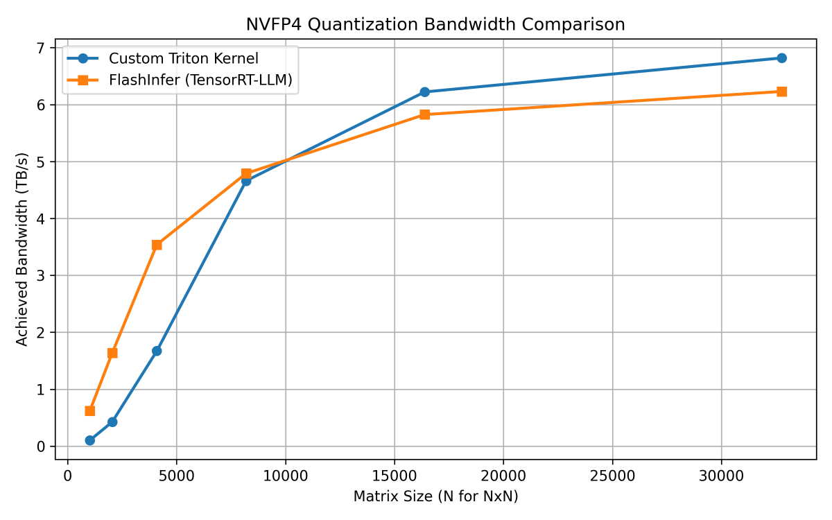
As you can see, the Triton kernel goes hand-in-hand with the optimized CUDA kernel when compared on a B200. For smaller shapes, the CUDA kernel is faster than Triton while for larger shapes, the Triton kernel outshines the CUDA kernel and almost touches 7 TB/s memory bandwidth.
This example goes to show that in less than 100 lines of carefully crafted Triton kernel with inline PTX, we can get to the same performance of an optimized CUDA kernel and sometimes even beat it, atleast for non-GEMM based workloads. Pretty cool, right?
Closing Thoughts
Inline elementwise PTX in Triton hits a really sweet spot. On one hand, you keep everything inside Python: the productivity, composability, and rapid iteration that made you choose Triton in the first place. On the other hand, you regain surgical control over instruction selection whether that’s bit packing, vectorized f16x2 math, approximate reciprocals, or special conversion operations like cvt.e2m1x2.f32 that Triton doesn’t expose directly today.
That said, this is not a silver bullet. It comes with some not-so-ignorable tradeoffs:
- You are responsible for correctness: register constraints, packing factors, and dtypes must line up perfectly.
- Debugging is harder: mis-specified constraints can silently produce wrong results.
- The abstraction leaks: your kernel becomes architecture-aware, and portability across vendors or even future NVIDIA architectures may require revisiting the PTX.
- You are limited to elementwise semantics: no shared memory, no explicit synchronization, no warp-level control.
If you need maximum flexibility, full control over memory hierarchies, warp-level gymnastics and so on, then dropping down to CUDA or NVIDIA’s CuTe DSL is still the right tool for the job. In practice, the most effective approach is often hybrid: write the bulk of the kernel in clean Triton, and inject PTX only where it truly matters. When used this way, inline elementwise PTX can turn Triton from a “high-level DSL” into a surprisingly sharp low-level tool, one that lets you compete with hand-optimized CUDA while still writing Python.
Thanks for reading!