
H3 Max: Built with fal Inference and Training

H3 Max generates a 5-second video in under 3 seconds. In our human preference evaluations against twelve leading video models, it ranks first on quality, prompt understanding, and aesthetics. Independent benchmarks from Artificial Analysis and Design Arena rank it first as well. We’ve written about the model itself. This article covers the platform that takes it from training to production and keeps performance optimized as demand grows.
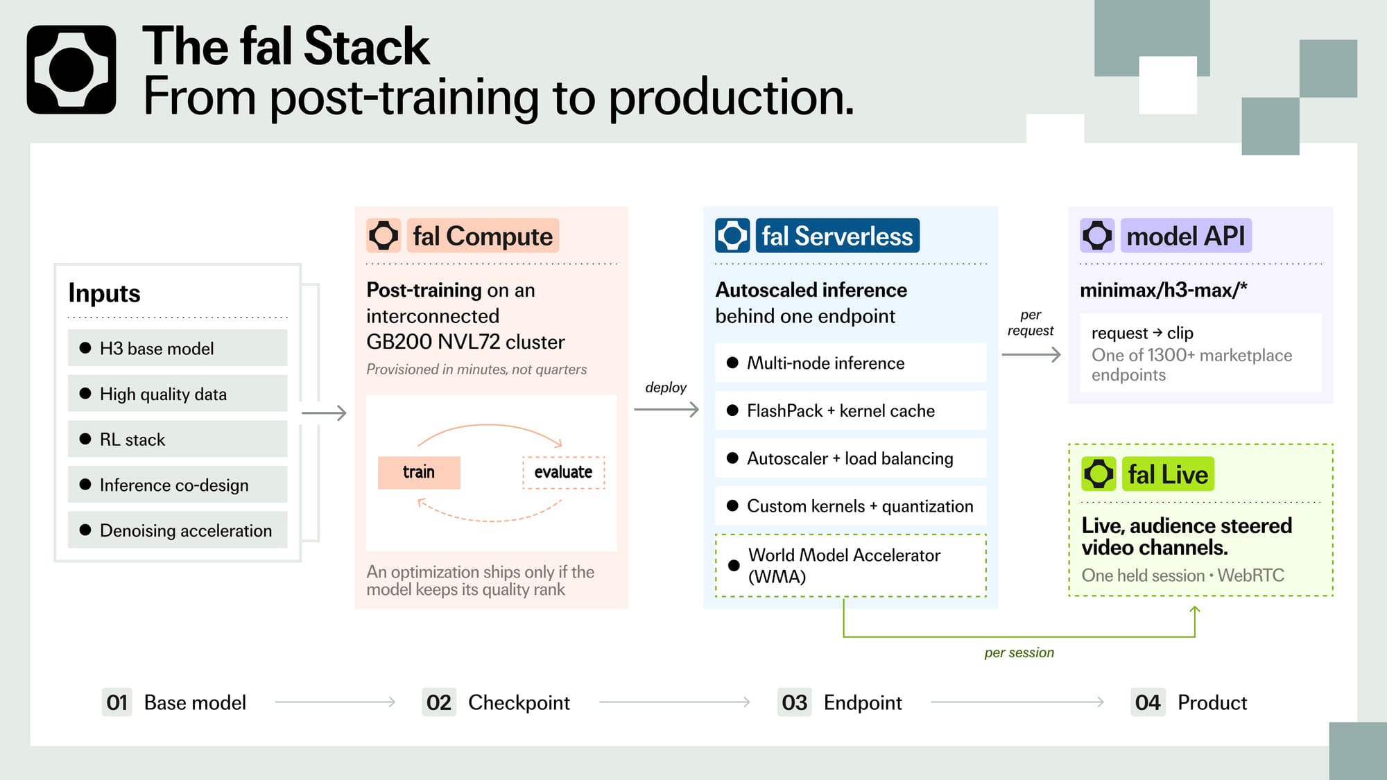
The fal platform is three layers that compound: fal Compute, fal Serverless, and fal Model APIs.
fal Compute provides the infrastructure for training: clusters of 16 or more nodes interconnected over RDMA fabrics such as InfiniBand or RoCE, rented for long-running training jobs.
fal Serverless is where trained models get deployed and served: billions of requests a day across thousands of endpoints. It got there because our own ML team has been dogfooding it for four years, and every reliability and observability feature exists because we needed it ourselves.
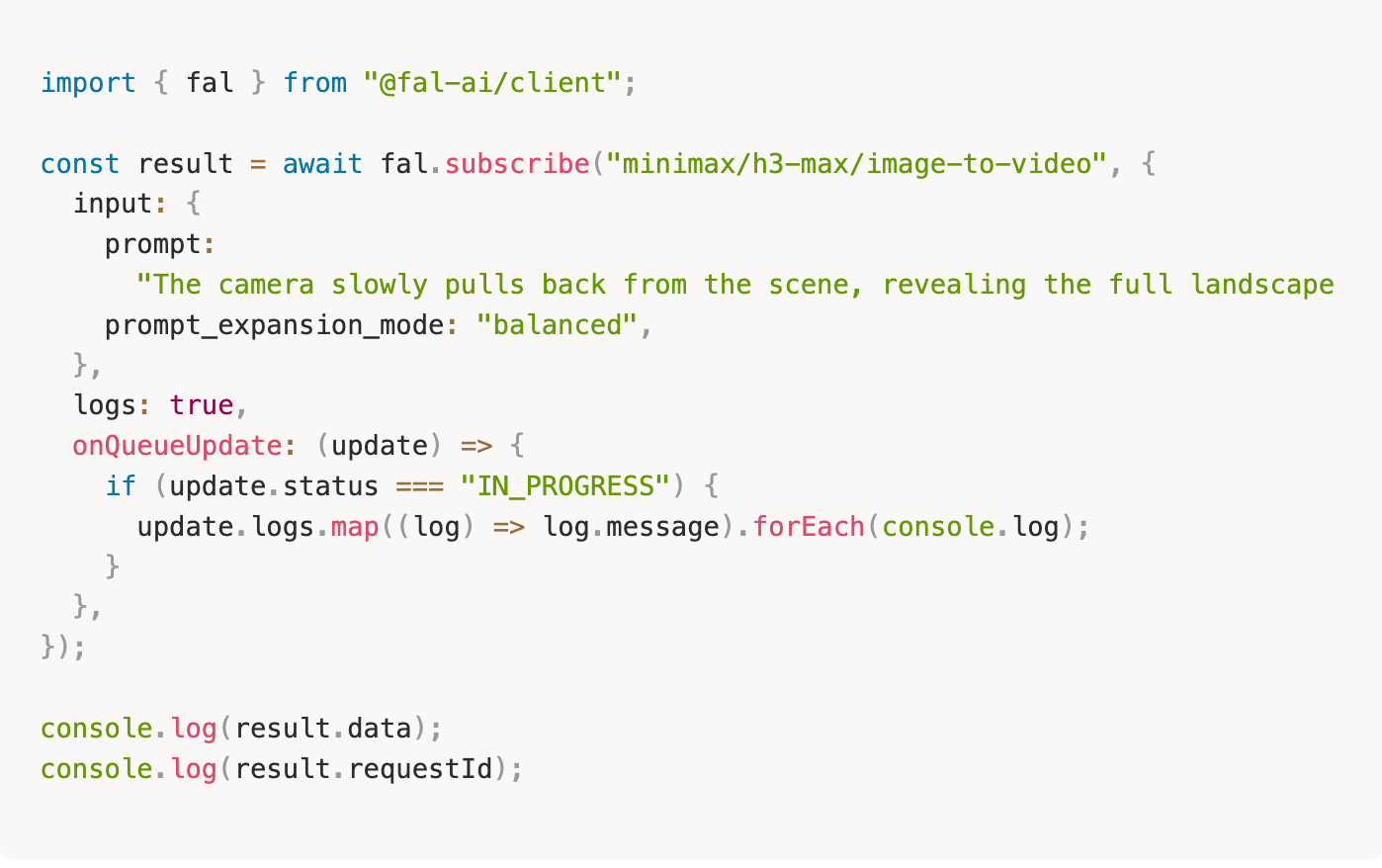
Model APIs sit on top: 1300+ endpoints behind a single API interface. When you call minimax/h3-max/image-to-video, you are hitting a Model API, and the queuing, autoscaling, and error handling underneath it are handled for you.
Many of our customers move along this stack in order: train on Compute, deploy on Serverless, then distribute as a Model API on the marketplace. H3 Max went through exactly this lifecycle. This article walks through it layer by layer, along with the techniques that let H3 Max deliver two different things that are easy to conflate. The first is low inference latency: how long one generation takes on a warm GPU that is already running. The second is low end-to-end latency at scale: how long a user actually waits for their video once queueing and cold starts are added on top of inference. The first is mostly a model problem. The second is an infrastructure problem, and it is the one Serverless exists to solve.
Moving towards low latency, high quality video generation
For a while, generative video models followed a predictable pattern: each new model understood prompts better and rendered more detail, but latency barely moved. Quality was the axis everyone optimized. The standard way to buy speed was to cut sampling steps or serve a smaller model, and the output got worse on the way down.
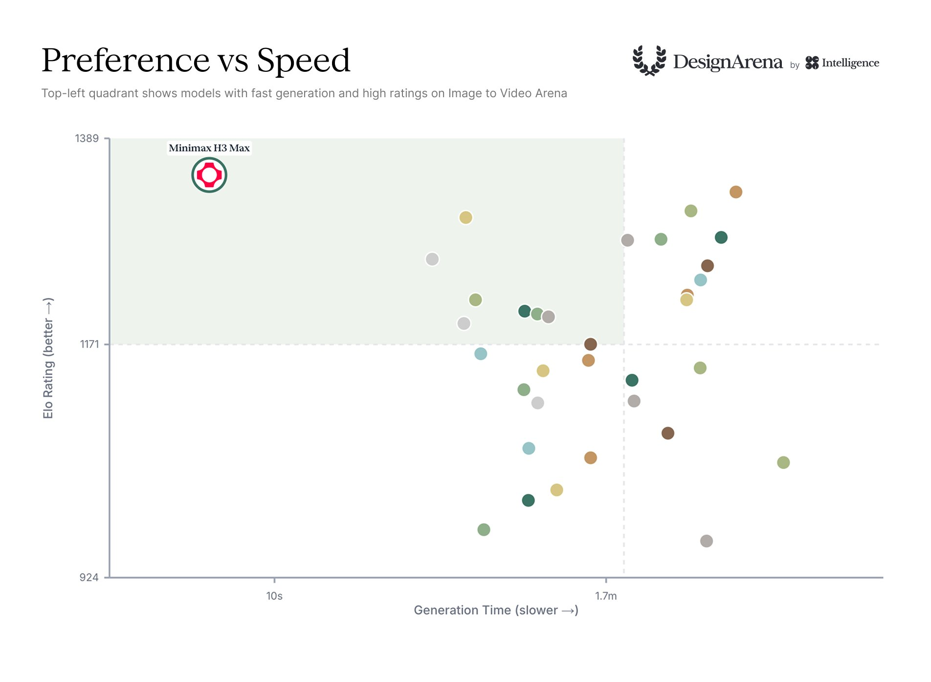
H3 Max is the first model in the industry to break through that barrier into a new zone: high quality and low latency at once. The chart above shows the first number from the introduction, inference latency. On the fal Serverless dashboard, it surfaces as Request Execution on the App Analytics tab, measured as the time spent executing the endpoint handler, which is inference plus whatever else the handler does.
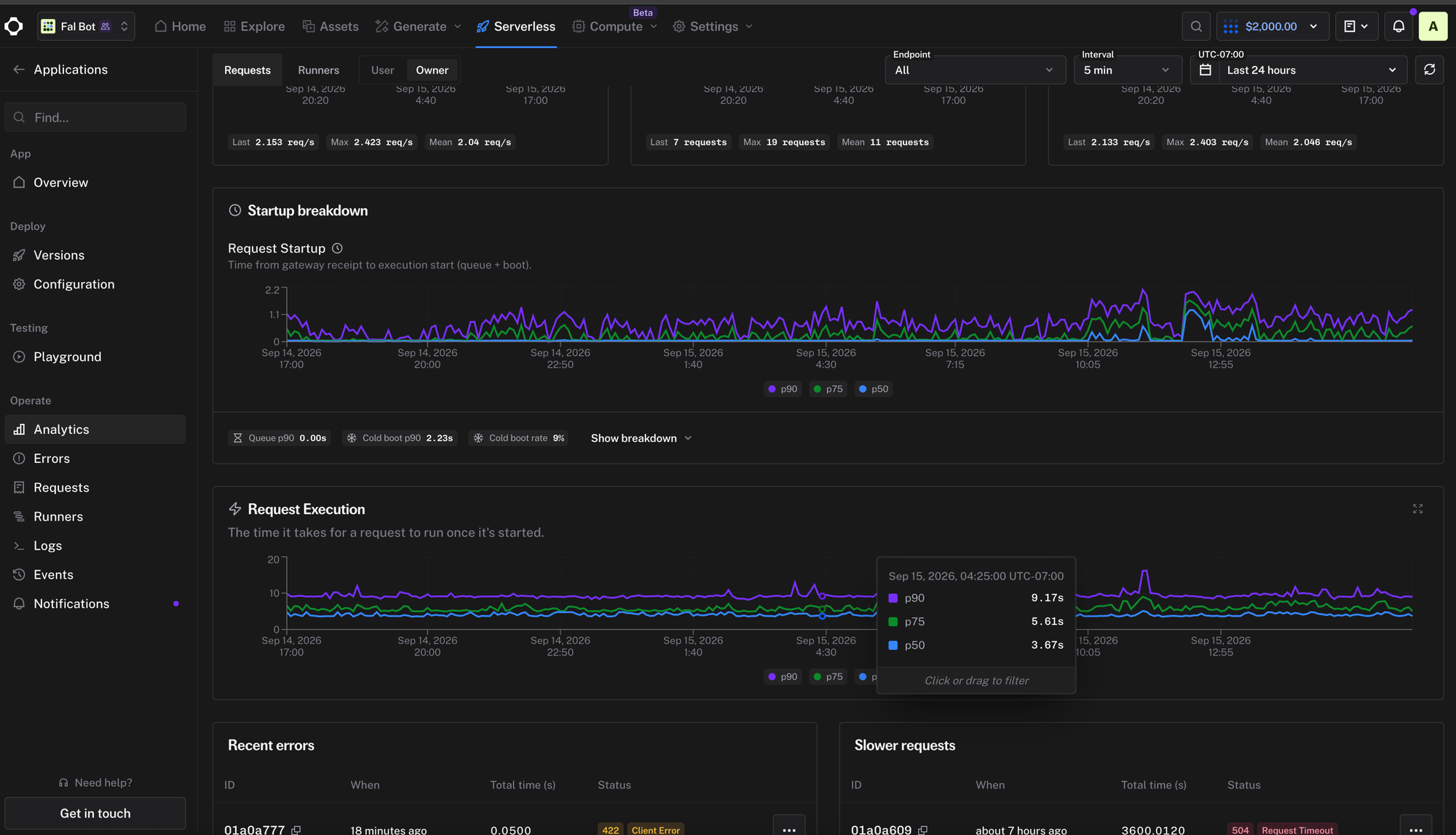
The second number is end-to-end latency at scale. When thousands of requests arrive at once, more than your idle capacity can absorb, the total time a user waits also includes queueing time and cold starts. The dashboard splits the parts into Request Startup and Request Execution, and measures the whole directly on the End-to-End Latency chart, timed per request from receipt to response. Keeping that number low under load is one goal of the Serverless product, and it is a different engineering problem from making a single generation fast.
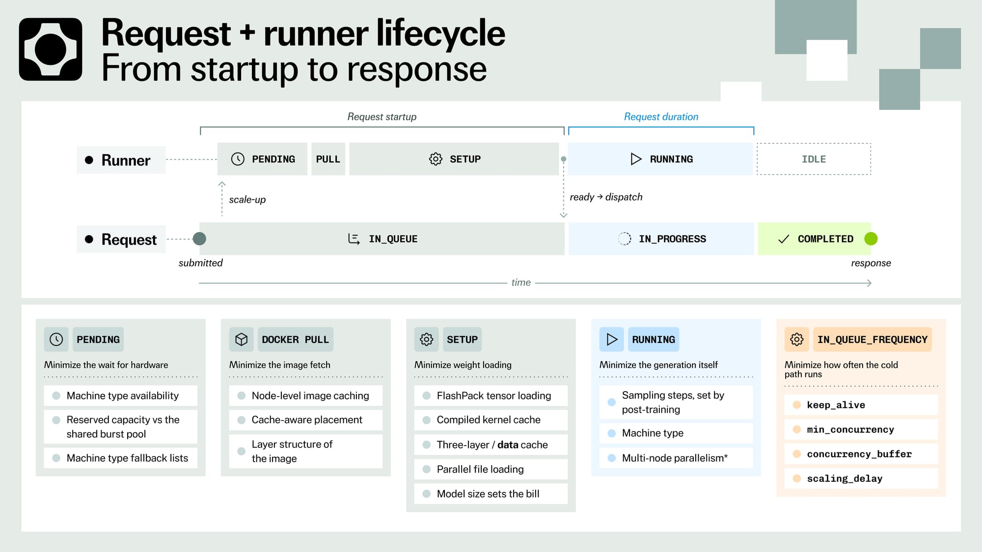
The diagram below shows how requests and runners connect. A request enters the queue, and if an idle runner exists it starts right away. If not, the request waits, and the autoscaler adds a runner if the scaling configuration allows it, below the max_concurrency and past the scaling delay. When a new runner is needed, its cold start becomes part of the request's startup time. The queue has no size limit, and retry-able runner failures are automatically re-queued, so bursts are absorbed rather than dropped.
Layer 1: Post-training H3 Max on fal Compute
We start at the training layer. H3 Max was post-trained by the fal Research team on fal Compute, with an explicit goal: minimize inference time while maximizing quality. On the end-to-end latency chart, this layer in particular moves Request Execution.
For a diffusion-based video model, inference time depends largely on the number of sampling steps and the cost of each step on the selected hardware. Post-training is where we reduced both. H3 Max used fal's post-training and reinforcement learning infrastructure for diffusion transformers, with high-quality training data, and we only shipped optimizations that preserved the model's ranking in our quality evaluations. Model size is different. It was fixed by the base model before any of this work, and it cascades through everything downstream: it determines the machine type, whether the model fits on one node or must be sharded across several, and how long weights take to load on a cold start.
The training itself ran on a cluster of interconnected GB200 NVL72 nodes on fal Compute. The final run took on the order of a week to ten days; considerably more time went into the experiments that shaped it. An optimization only shipped if the model kept its rank in our quality evaluations. There are plenty of ways to make a video model faster that look excellent on a latency chart and quietly cost you the output. Those were rejected.
fal Compute is the same product any team can rent: interconnected clusters, typically 16 nodes and up, with full control of the machines. If your training job outgrows a single node, this is the layer built for it.
Layer 2: Inference at scale with fal Serverless
So you have trained (or post-trained) a model. Next is deploying it to serve inference at scale, with the goal of minimizing end-to-end latency. fal Serverless gives you a set of levers over both halves of the split from the last section, Request Startup and Request Execution.
Reducing cold start impact
Start with the part everyone feels first: the cold start. Opening any runner on the Serverless runners page shows its side-sheet, with the cold start broken into stages:
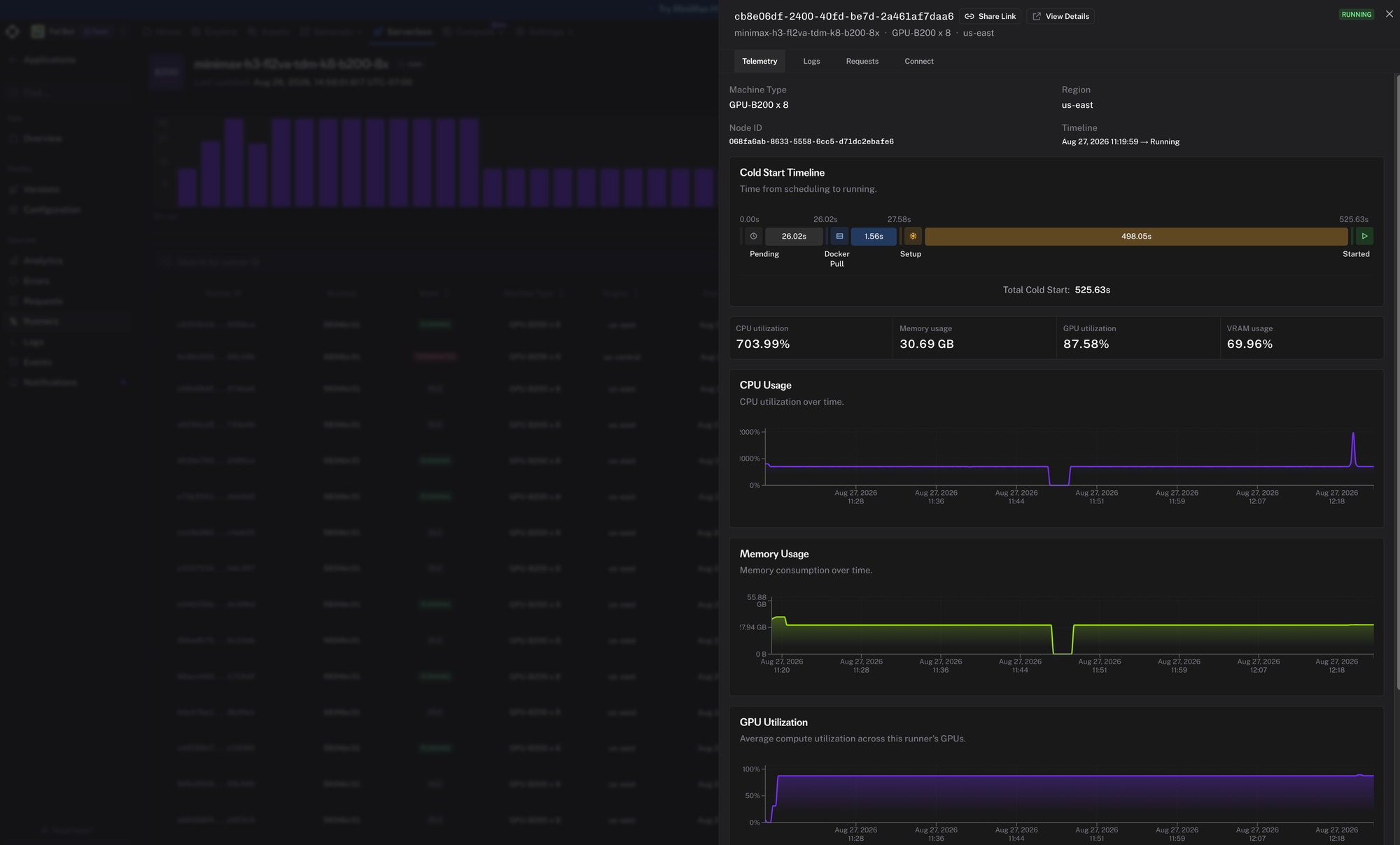
That breakdown tells you where to aim. A runner moves through five key states on its way to serving traffic and the time from PENDING to IDLE is your cold start latency.
PENDING: waiting to be scheduled onto available hardware. fal absorbs this stage and does not bill for it.DOCKER_PULL: the environment image is pulled to the node and cached. This stage is skipped entirely when the node already holds the image, and it is not billed either.SETUP: the container runs your application'ssetup()function, loading model weights onto the GPU and doing any other startup work. Billing starts here.IDLE: ready to serve requests, not actively executing a generation.RUNNING: actively executing a generation.
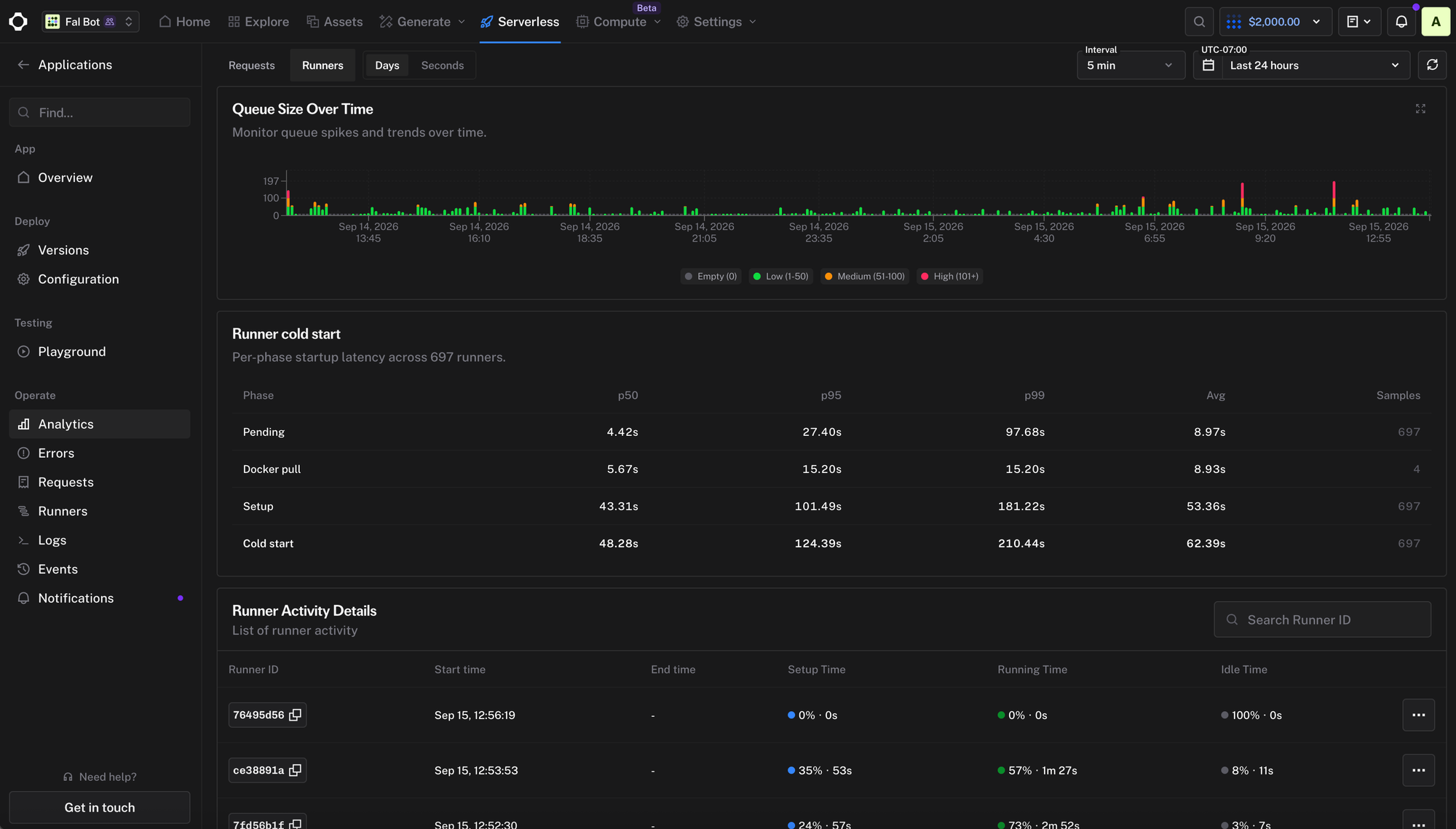
The side-sheet above shows a single runner. The Runners tab also aggregates cold starts across all runners in the selected range, with p50, p95, p99, and average duration per state. One slow runner can be an outlier, so this is the view that shows which state actually contributes most to cold start latency. The sections below go through those states one at a time.
Getting capacity when you need it
PENDING is the wait for hardware, so minimizing it comes down to how many free machines exist of the machine_type your app configures. Enterprise customers of fal Serverless typically structure capacity in two tiers:
- A reservation: a fixed number of GPUs per machine type, held 24/7 and isolated from the shared pool. Reserved capacity eliminates pending and setup time for a guaranteed pool of GPUs, which in practice means always-warm runners, no cold starts on the reserved floor, and predictable unit economics.
- Bursting above that baseline into the shared pool. The burst pool is shared across Enterprise customers, so performance there is less predictable: under contention, a burst can wait longer in
PENDINGthan reserved capacity ever does. Pricing differs too. Reservation rates are fixed by contract, while non-contracted usage is billed at prevailing rates, which can change. However, the burst mechanism provides elasticity and flexibility that make the Serverless product even more beneficial during high-traffic periods, model launches and experiments, on top of your baseline reservation.

H3 Max does something additionally clever. It load balances across multiple machine types by following the multi-app-routing pattern. The public endpoint is a small CPU app that owns everything about a request that does not need a GPU: validation, prompt expansion, the safety checker, billing. The generations run on separate GPU apps on different machine types, each scaling independently.
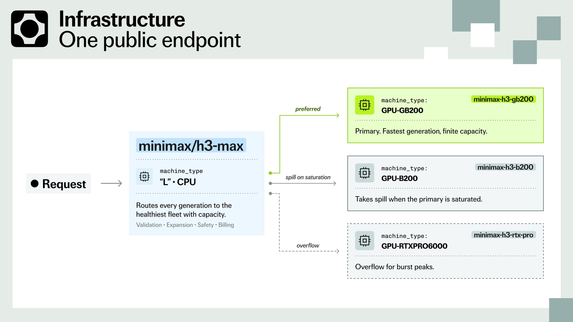
Any single GPU fleet has finite capacity. When a spike exceeds what the fastest fleet can absorb, the choice is to queue or to generate on another fleet, and the router takes the second option. The routing itself is application code rather than a platform feature: the CPU app knows each fleet's capacity, which is its runner count, and tracks how many generations are in flight on each one. Every request goes to the most preferred fleet with a free slot, so when the fastest fleet fills up, requests spill to the next one, and when it has room again, traffic moves straight back. A fleet with a rising error rate gets deprioritized until the errors stop, and if every fleet is full at once, requests queue rather than fail.
This is different from fallback machine types, where a single app lists machine types to try in order when a runner boots. Fallbacks solve hardware availability at scale-up. Routing decides where each request goes while it is in flight.
Minimizing image pull time
Before a runner can execute your setup(), the node needs your container image. Often this stage costs nothing: images are cached on the machines themselves, the scheduler prefers nodes that already hold your image, and a runner placed on one skips the pull entirely, showing ‘Cached’ on the runners page instead of a duration. When a pull does happen, it is layered, so only the layers you changed come over the wire. That is why the side-sheet example earlier spent just 1.56 seconds in DOCKER_PULL, and the container image optimization guide covers how to keep it that way. For an app like H3 Max serving continuous traffic, the pull is either skipped or a rounding error next to setup.
Minimizing setup time
In the side-sheet example, setup was 496 seconds of a 524-second cold start, and that ratio is typical. Loading tens of gigabytes of weights onto a GPU is the expensive part of starting any large model. It is also the part the platform has the most machinery for. FlashPack, fal's open-source tensor loader, streams weights from disk to GPU at up to 25 Gbps without GDS, and H3 Max ships every component this way: the transformer, both VAEs, and the text encoder. Compiled kernel caching means the first runner compiles its torch.compile kernels and every runner after it loads the result instead of recompiling. And underneath both, the /data filesystem is a three-layer cache, local NVMe, a datacenter-wide cache, then the object store, so cold starts get faster on their own as an app takes traffic and the caches warm.
Optimizing the autoscaler configuration
Faster cold starts help when you need a new runner. Keeping enough runners ready can avoid that wait altogether. Four settings control how much capacity stays available and when Serverless adds more.
min_concurrencymaintains a minimum number of runners.concurrency_bufferkeeps spare runners available above current demand.keep_alivecontrols how long an idle runner stays active.scaling_delaydelays scale-up so brief traffic spikes do not immediately create new runners.
You can adjust all four on a running app without redeploying. That lets you tune capacity as you see how people use your product, rather than having to predict the traffic pattern before launch. What Is a Serverless GPU Cold Start? covers the settings in more detail.
Minimizing inference latency
Two major factors shape the model’s generation time (Request Execution). The first is the model: how many sampling steps it takes and how much computation each step costs, which the training procedure sets. The second is the hardware those steps run on. On Serverless you choose the machine type, from Hopper-generation GPUs to Blackwells, and a single app can run multi-GPU inference, up to 8 GPUs in one node.
With H3 Max this is taken a step further with multi-node inference: running a single app across multiple GPU nodes, presented as one deployment behind one endpoint. Every node loads its share of the model, and the leader node serves requests. H3 Max serves this way on GB200s, because a model of this size does not fit comfortably on one node.
fal's ML team further optimized inference latency with Falcon, fal's in-house inference engine. It is the library our apps import to execute a model on the GPU, with the kernels, quantization, and compilation that decide how fast each sampling step runs. We ported H3 from sglang to Falcon, and it is part of what keeps Request Execution low on every machine type we serve. For larger contracts, our kernel engineers can apply the same work to your model.
Observing metrics in production
Every stage this article has walked through shows up as a metric on the Serverless dashboard: queue wait, each cold start stage, the inference itself. When a request feels slow, the breakdown shows which stage is responsible. There is no special internal tooling behind any of it. Every app you deploy gets the same dashboard we use to run H3 Max.
App Analytics is the aggregate view: throughput, error rates, and latency percentiles split into Request Startup and Request Execution, so you can see at a glance where the time is going. Runner Analytics is the per-runner view: the side-sheet from earlier, plus live GPU telemetry and logs filtered to that runner. For teams with their own observability stack, OpenTelemetry traces and log drains export the same data.
Observability on fal is also not read-only. The same dashboard is where you adjust the scaling configuration of a running app: machine type and the scaling parameters change live, with no redeploy, and persist across future deployments. You diagnose and fix in the same place.
Here is what those views look like on H3 Max itself:


Pushing the realtime boundary further with fal Serverless WMA
Everything above assumes a request and a response: you ask for a clip, you get a clip. Interactive, realtime applications do not work that way. A voice agent responds mid-conversation. A playable world updates as you act in it. A live video stream changes in response to its viewers. These applications need a session that stays open, output that never stops, and input that lands immediately. A queue hop plus a startup on every request cannot deliver that.
WMA, the World Model Accelerator is fal's Serverless primitive for serving interactive models over WebRTC, the protocol video calls use. The client connects once through the wma.fal.run bridge, and from then on the runner holds a live session: media streams straight to the client, and control messages ride back on a data channel.
Why not plain requests, or a WebSocket? A request returns a finished clip. You submit, you wait, you download. That is the right shape for one video and the wrong shape for a continuous stream. A WebSocket holds a connection, but it runs on TCP, where one lost packet stalls every frame behind it, and it delivers raw payloads, so your app has to decode frames, pace playback, and keep audio in sync itself. WebRTC hands the browser a media track instead. You attach it to a video element and the browser does hardware decode, pacing, and audio-video sync natively, skipping lost frames rather than stalling on them. After the handshake, media can flow directly between the runner and the client. The same session works for any realtime model, not just video. A voice model streams an audio track, an image or 3D model streams its frames as a video track, and structured state - actions, poses, scene updates - goes over the data channel.
The developer surface makes the abstraction concrete. This is the docs' minimal world model, complete except for the inference function you would supply:
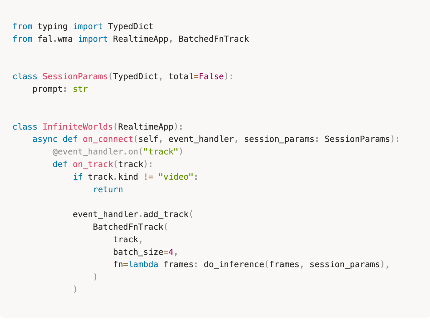
fal.live is one example of a product running in production today: continuously broadcasting channels of AI video and audio, steered live by their audience. Each channel is one WMA session, and viewers watch a broadcast of it, so a channel costs the same GPU at ten viewers or ten thousand. A ‘winning’ prompt travels over the open connection and changes the stream within seconds, where before it would have been a new request with a queue hop and a poll.
This is what fal Serverless enables with WMA: realtime applications at very low latency, with the infrastructure abstracted away. A WMA app deploys like any other Serverless app, so you get the same playground, dashboard, and analytics without building session management, deployment, or monitoring yourself.
Layer 3: Distribution through the Model API
The last step of the lifecycle is distribution, and it is the layer most people know fal by. Every Model API on fal, H3 Max included, is a Serverless app running in shared auth mode, on the same runners, caching, and analytics you saw above. That makes this the smallest technical step in the whole stack. Once shared mode is enabled on your account, setting app_auth = "shared" lets other fal users call your app. Publishing also involves configuring billing and working with the fal team on the marketplace listing, while retaining your existing inference implementation.
In shared mode, callers authenticate with their own fal API key, and you stay in control of how usage is billed. Your app reports billable units on each response, so you decide whether a request is priced per image, per megapixel, per second of generated video, or flat, and the platform meters callers accordingly. The publishing guide covers the mechanics. The fal team configures the model card and the per-unit price with you, and callers see that price on your model's page.
What publishing buys is distribution. Your model becomes one of the 1300+ endpoints developers already integrate, in front of fal's existing customer base, and you get paid when other people's applications call it. There is no serving stack to build and no separate billing system to run. H3 Max lives there today as minimax/h3-max/image-to-video and minimax/h3-max/text-to-video, and the day your model is ready, it can live there the same way.
One lifecycle, and where it goes
Step back and the three layers are one path walked in order. H3 Max was post-trained on Compute, on an interconnected GB200 cluster, until it held first-place quality at faster-than-realtime speed. It was deployed on Serverless, where multi-node inference, FlashPack, kernel caching, and the scaling parameters keep both halves of its latency low, and where the same dashboards we used to tune it are the ones any customer gets. And it is distributed as a Model API, one endpoint among 1300+, callable with the TypeScript snippet at the top of this page. Nothing in that path is reserved for fal's own models. It is the product, end to end.
Our hypothesis about what comes next is simple: the two curves that meet in this model are not moving at the same speed. Video model quality is approaching the flat part of its curve, where each generation of models buys a slightly better-understood prompt and a slightly cleaner frame. The cost of serving that quality is nowhere near its floor. Hardware improves, kernels improve, serving systems improve, and each of those compounds the others, so the price of a generation keeps falling after quality gains have gone marginal.
H3 Max is the first model where generation runs faster than playback at frontier quality, which makes it the first glimpse of what that crossover produces: video you iterate on rather than wait for, and beyond that, applications that generate continuously, interactive video that responds to its audience, worlds rendered as they are explored. That infrastructure already exists: WMA, the interface fal.live broadcasts on, is available today, and it is the layer we expect the next frontier of generative media to be built on. Running a model like that continuously is expensive today. It will not stay expensive. The teams building for that moment are starting now, and they are walking the same path this article just walked: training on Compute, deploying on Serverless, and distributing as Model APIs.
That is the bet the fal stack makes.
Get started
Everything above is available today. Pick the entry point that matches where you are:
- If you have a model to serve, deploy it on fal Serverless. Same runners, same caching, same dashboards as H3 Max.
- If you want to see the dashboards first, explore the read-only demo: a demo account with the runner timelines and analytics this article walked through. You need a fal account to open it.
- If you just want the model, H3 Max is in the playground, or call it with the snippet at the top of this page.
- If you are training or going realtime, talk to us about Compute, or build on WMA for live sessions.